The Origins of EV: Polarization EV and Polarizability EV

Author: Sigma (Twitter: @sigm_4)

What This Article Covers

• Among the factors that compose EV are range EQ, position, the degree to which a range is polarized, and how much a range will polarize in future streets.

• As a toy model that lets us tune how much a range will polarize in the future, we devise the beta-[0, 1] model.

• We estimate how much future polarization potential actually exists in real poker, and compare it with the model.

The Origins of EV

In this chapter, we review what factors generate EV under Nash equilibrium (i.e., when both players play rationally with full knowledge of each other's ranges).

EV in the Half-Street Game: Equity EV and Polarization EV

First, let us think about what kind of range yields greater EV in a half-street game (i.e., when only one player holds the right to bet). For example, on the river when you are IP, what kind of range would you be happy to hold?

Naturally, holding only the nuts would be ideal. Generalizing slightly, the higher your range's EQ, the higher your range EV is expected to be. Let us call the EV generated by range EQ the equity EV (we deliberately write out "equity" rather than "EQ EV," which would be hard to read).

Formally, we define equity EV as the current pot distributed according to range EQ.

But of course, range EQ is not the only thing that composes EV.

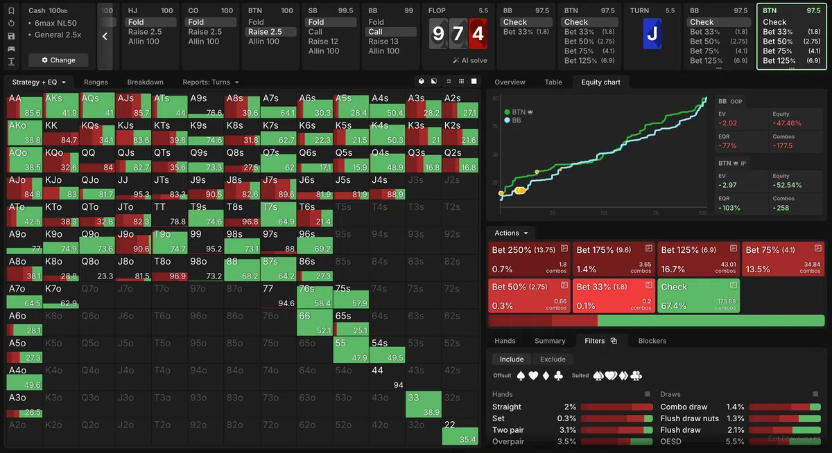
As a simple example, let us look at the following spot [Figure 1]. Figure 1 is a BTN vs. BB SRP on KsQh5d-7h-As that has proceeded xb 125%c-xb125%c-x. (Note: all solutions presented hereafter are based on GTO Wizard Cash 100bb 6max NL50 2.5x-GTO.)

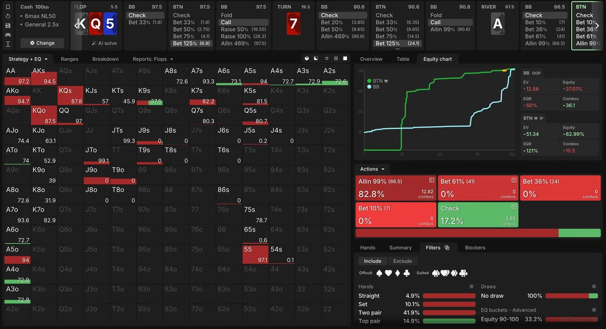
Looking at Figure 1, the EQs of BTN and BB are 62.99% and 37.01%, respectively. Meanwhile, the EVs of BTN and BB are 76.06% and 18.61% of the pot, respectively (they do not sum to 100% because of rake). BTN's EV is about 13 pt. higher than its EQ. What causes this difference?

Looking at the EQ graph, we see that BTN's range is polarized relative to BB. Exploiting this polarized range, BTN appears to earn EV by betting (all in) with high-EQ and low-EQ hands so as to squeeze BB's marginal range from both sides.

Such a situation is well described by the so-called AKQ model. Matching the situation above, suppose IP holds A or Q with probability 63% and 37% respectively, and OOP holds K with probability 100%. Then IP's EQ is 63%, closely resembling the situation in Figure 1. In the Nash equilibrium of a half-street game where only IP is allowed a pot bet, IP bets A and Q in a 2:1 ratio and captures 94.5% of the pot in EV [Figure 2].

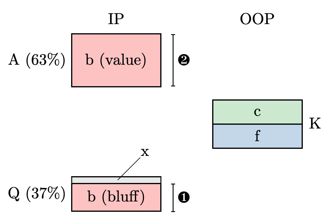
In other words, in this model, IP's polarized range allows it to capture more EV than its range EQ alone would indicate. We call the EV generated by the degree of range polarization the polarization EV in this article (in some circles, the term distribution EV is used).

In this AKQ model case, (IP's EV) = (Equity EV) + (Polarization EV). Concretely, the breakdown is 0.945 = 0.63 + 0.315.

In the actual case of Figure 1, compared with this AKQ model, IP's range is less polarized (IP has a smaller proportion of trash hands than the model, while its high-EQ hand distribution is closer to OOP's), so we can interpret BTN's polarization EV as smaller and the total EV obtained as smaller.

As an extreme case, even when range EQ is exactly equal for both players, total EV can still be obtained through polarization EV. This is realized in the (most commonly seen) AKQ model where the ratio of A to Q is 1:1. In this case both players hold 50% EQ, but the AQ side captures 3/4 of the pot as total EV (when only a pot bet is allowed), corresponding to its overall range bet frequency. Here, the polarization EV equals one half of the equity EV. Furthermore, if we increase the bet size to infinity, in the limit the polarization EV becomes equal to the equity EV. One of the lessons of the AKQ model was precisely this polarization EV.

Here, we note that polarization EV does not have any rigorous definition. However, if we dare to define it relatively rigorously, it would be as follows.

(Polarization EV) = [(EV lost when the two ranges are swapped) − (equity EV lost in the swap)] / 2

Under this definition, if the two ranges are exactly identical, the polarization EV is trivially 0.

Note: For example, consider a half-street game where both players hold A, K, and Q. The equity EV is 50% of the pot and the polarization EV is 0. However, the player granted the right to bet can obtain an additional finite EV. Such EV from the asymmetry of action certainly exists, but since it does not contribute to the EV split at the start of each street in real poker, we will not delve into it here.

EV in the Full-Street Game: Position EV

So far, through the half-street game, we have seen two factors that generate EV: range EQ and polarization. Now let us consider expanding the game from half-street to full-street—that is, the case where OOP and IP are each given one chance to bet. Here too, range EQ and polarization still affect EV. But that is not all. The quality of each player's position also affects EV—that is, whether one is OOP or IP.

To see this, let us look at the full-street [0, 1] model.

Full-street [0, 1] model
- OOP and IP each independently draw one real number from the uniform distribution on the closed interval $[0, 1]$.
- OOP can bet (or check) first, and if OOP checks, IP can also bet (or check) (= full-street).
- Both players choose call or fold against the opponent's bet; raising is not allowed.
- The pot size is 1, and the bet size is fixed at the pot size (= 1).
- When one player's bet is called by the other, or when both players check, a showdown occurs, and the player who drew the larger real number wins the current pot.

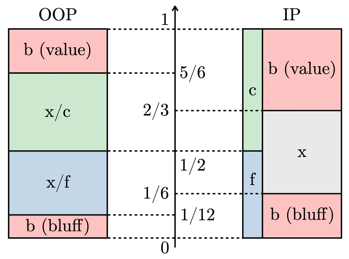
For the Nash equilibrium of the model with a general bet size, please refer to this article. In outline, the Nash equilibrium is as follows: OOP makes polarized bets using high-EQ and low-EQ hands, and against OOP's check, IP likewise makes polarized bets using high-EQ and low-EQ hands. Figure 3 illustrates this Nash equilibrium.

What is important here is that IP can lower its value-bet threshold and bet with more hands than OOP. Because OOP has already siphoned off its high-EQ hands into betting, IP can more efficiently attack OOP's condensed check range. As a result, IP obtains greater EV than OOP.

Note: This model also has another Nash equilibrium that is not a threshold strategy, but we omit it here.

When the bet size is fixed at the pot size, the EVs of IP and OOP are 13/24 and 11/24, respectively. Since both ranges are exactly identical, the equity EV is 1/2 for both IP and OOP, and the polarization EV is 0. Thus, the remaining part of the EV can be regarded as arising from the difference in position. Let us call this the position EV. That is, in a full-street game, (Total EV) = (Equity EV) + (Polarization EV) + (Position EV). For the full-street [0,1] model with bet size 1, the breakdown for IP is 13/24 = 1/2 + 0 + 1/24.

If we were to formally define position EV as well, the natural way would be the following.

(Position EV) = (EV lost when only the positions are swapped, keeping the ranges as is) / 2

Let us summarize the definitions of equity EV, polarization EV, and position EV introduced so far, rewritten for the full-street case.

• (Equity EV) = (Pot) × (range EQ [%]) / 100

• (Polarization EV) = [(EV lost when only the ranges are swapped, keeping the positions as is) − (equity EV lost in the swap)] / 2

• (Position EV) = (EV lost when only the positions are swapped, keeping the ranges as is) / 2

By way of review, let us look at two examples.

Example 1: Full-Street AKQ Model

Earlier we looked at the AKQ model as a half-street game; as a relatively straightforward application, let us check the full-street AKQ model. Here, we fix the bet size at the pot size. The model details are as follows.

Full-street AKQ model
- OOP player: Holds K.
- IP player: Holds A or Q with equal probability.
- OOP can bet (or check) first, and if OOP checks, IP can also bet (or check) (= full-street).
- Against the opponent's bet, the options are call or fold; raising is not allowed.
- The pot size is 1, and the bet size is fixed at the pot size (= 1).
- When OOP checks or IP calls, a showdown occurs, and the player with the higher-ranking card wins the current pot.

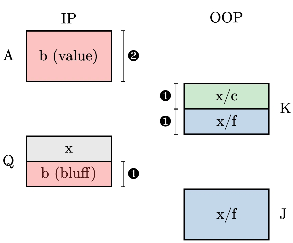
As is well known, the Nash equilibrium of this model is: OOP holding K always checks, and IP bets all of its A and half of its Q. Let us denote the EVs that OOP and IP obtain, making the range composition explicit, as $\mathrm{EV}^{\mathrm{OOP,\,K}},\; \mathrm{EV}^{\mathrm{IP,\,AQ}}$. Concretely:

$$ \begin{align*} \mathrm{EV}^{\mathrm{OOP,\, K}} &= \frac{1}{4} \quad\quad (1) \\ \mathrm{EV}^{\mathrm{IP,\, AQ}} &= \frac{3}{4} \quad\quad (2) \end{align*} $$

Below, we decompose both players' EVs into equity EV, polarization EV, and position EV.

First, since each player's range EQ is 50%, the equity EVs of OOP and IP are each

$$ \begin{align*} \mathrm{EV}^{\mathrm{OOP,\,K}}_{\mathrm{equity}} = \mathrm{EV}^{\mathrm{IP,\,AQ}}_{\mathrm{equity}} = \frac{1}{2} \quad\quad (3) \end{align*} $$

Next, to compute the polarization EV, we swap only the ranges while keeping positions fixed. In the Nash equilibrium where OOP is given A and Q and IP is given K, the AQ side, as before the swap, always bets A and bets Q at a rate of 1/2. The K side checks back after the AQ side's check, ending the hand. Therefore, regardless of the swap, the side holding AQ gets 3/4 and the side holding K gets 1/4. That is,

$$ \begin{align*} \mathrm{EV}^{\mathrm{OOP,\,K}} &= \mathrm{EV}^{\mathrm{IP,\,K}} = \frac{1}{4} \quad\quad (4) \\ \mathrm{EV}^{\mathrm{IP,\,AQ}} &= \mathrm{EV}^{\mathrm{OOP,\,AQ}} = \frac{3}{4} \quad\quad (5) \end{align*} $$

From this, the respective polarization EVs of OOP and IP are computed as

$$ \begin{align*} \mathrm{EV}^{\mathrm{OOP,\,K}}_{\mathrm{polarization}} &= (\mathrm{EV}^{\mathrm{OOP,\,K}}-\mathrm{EV}^{\mathrm{OOP,\,AQ}})/2 = -\frac{1}{4} \quad\quad (6) \\ \mathrm{EV}^{\mathrm{IP,\,AQ}}_{\mathrm{polarization}} &= (\mathrm{EV}^{\mathrm{IP,\,AQ}}-\mathrm{EV}^{\mathrm{IP,\,K}})/2 = \frac{1}{4} \quad\quad (7) \end{align*} $$

And the position EV can be computed by swapping only the positions while keeping the ranges fixed and taking the EV difference. That is, the respective position EVs of OOP and IP are

$$ \begin{align*} \mathrm{EV}^{\mathrm{OOP,\,K}}_{\mathrm{position}} &= (\mathrm{EV}^{\mathrm{OOP,\,K}}-\mathrm{EV}^{\mathrm{IP,\,K}})/2 = 0 \quad\quad (8) \\ \mathrm{EV}^{\mathrm{IP,\,AQ}}_{\mathrm{position}} &= (\mathrm{EV}^{\mathrm{IP,\,AQ}}-\mathrm{EV}^{\mathrm{OOP,\,AQ}})/2 = 0 \quad\quad (9) \end{align*} $$

Putting it all together,

$$ \begin{align*} \mathrm{EV}^{\mathrm{OOP,\,K}} &= \mathrm{EV}^{\mathrm{OOP,\,K}}_{\mathrm{equity}} +\mathrm{EV}^{\mathrm{OOP,\,K}}_{\mathrm{polarization}} +\mathrm{EV}^{\mathrm{OOP,\,K}}_{\mathrm{position}} = \frac{1}{2} - \frac{1}{4} + 0 \quad\quad (10) \\ \mathrm{EV}^{\mathrm{IP,\,AQ}} &= \mathrm{EV}^{\mathrm{IP,\,AQ}}_{\mathrm{equity}} +\mathrm{EV}^{\mathrm{IP,\,AQ}}_{\mathrm{polarization}} +\mathrm{EV}^{\mathrm{IP,\,AQ}}_{\mathrm{position}} = \frac{1}{2} + \frac{1}{4} + 0 \quad\quad (11) \end{align*} $$

Example 2: Full-Street AKQJ Model

The examples so far were cases where one of equity EV, polarization EV, or position EV was equal between the two players or was 0. Finally, let us close this chapter by looking at a more advanced AKQJ model in which all three differ between the players. The full-street AKQJ model is as follows.

Full-street AKQJ model
- OOP player: Holds K or J with equal probability.
- IP player: Holds A or Q with equal probability.
- OOP can bet (or check) first, and if OOP checks, IP can also bet (or check) (= full-street).
- Against the opponent's bet, the options are call or fold; raising is not allowed.
- The pot size is 1, and the bet size is fixed at the pot size (= 1).
- When OOP checks or IP calls, a showdown occurs, and the player with the higher-ranking card wins the current pot.

This is almost the same as the AKQ model, except that the OOP player now holds K or J rather than just K. The Nash equilibrium of this model is similar to the AKQ model: OOP checks its entire range, and IP always bets A and bets Q at a rate of 1/2. Figure 4 illustrates this Nash equilibrium. The EVs of OOP and IP are, respectively,

$$ \begin{align*} \mathrm{EV}^{\mathrm{OOP,\,KJ}} &= \frac{1}{8} \quad\quad (12) \\ \mathrm{EV}^{\mathrm{IP,\,AQ}} &= \frac{7}{8} \quad\quad (13) \end{align*} $$

Let us again decompose these into equity EV, polarization EV, and position EV. First, the equity EV is simple: since OOP and IP have range EQs of 25% and 75% respectively,

$$ \begin{align*} \mathrm{EV}^{\mathrm{OOP,\,KJ}}_{\mathrm{equity}} &= \frac{1}{4} \quad\quad (14) \\ \mathrm{EV}^{\mathrm{IP,\,AQ}}_{\mathrm{equity}} &= \frac{3}{4} \quad\quad (15) \end{align*} $$

Next, to compute the polarization EV, we consider swapping the ranges. The Nash equilibrium when OOP holds A or Q and IP holds K or J is quite different from the original model. The Nash equilibrium after the range swap is as follows.

First, OOP holding A or Q bets 4/5 of its A and checks 1/5, and bets 2/5 of its Q and checks 3/5. Against OOP's bet, IP calls 3/5 of its K and folds 2/5, and always folds J. When OOP checks, IP bets 2/5 of its K and checks 3/5, and bets 1/5 of its J and checks 4/5. Against IP's bet, OOP always calls A, and calls 1/3 of its Q and folds 2/3. Figure 5 illustrates this Nash equilibrium.

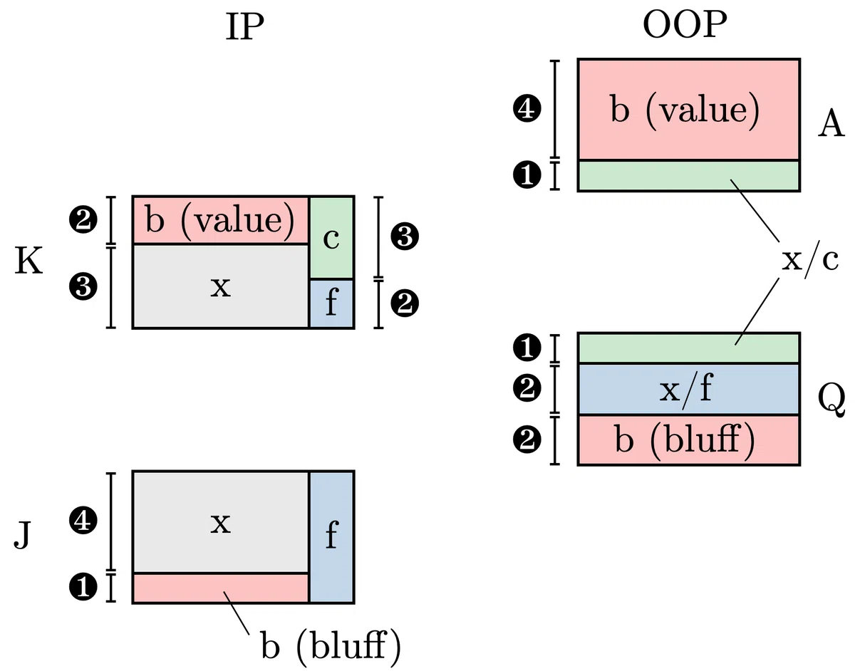
In other words, if OOP holding A or Q uses too much of its A for betting, its check range becomes too weak, so it appropriately keeps A in its check range to make IP's K (and J) indifferent between betting and checking. The EVs of OOP and IP after the swap are, respectively,

$$ \begin{align*} \mathrm{EV}^{\mathrm{OOP,\,AQ}} &= \frac{17}{20} \quad\quad (16) \\ \mathrm{EV}^{\mathrm{IP,\,KJ}} &= \frac{3}{20} \quad\quad (17) \end{align*} $$

Therefore, the respective polarization EVs of OOP and IP are computed as

$$ \begin{align*} \mathrm{EV}^{\mathrm{OOP,\,KJ}}_{\mathrm{polarization}} &= [(\mathrm{EV}^{\mathrm{OOP,\,KJ}}-\mathrm{EV}^{\mathrm{OOP,\,AQ}})-(\mathrm{EV}^{\mathrm{OOP,\,KJ}}_{\mathrm{equity}}-\mathrm{EV}^{\mathrm{OOP,\,AQ}}_{\mathrm{equity}})]/2 = -\frac{9}{80} \quad\quad (18) \\ \mathrm{EV}^{\mathrm{IP,\,AQ}}_{\mathrm{polarization}} &= [(\mathrm{EV}^{\mathrm{IP,\,AQ}}-\mathrm{EV}^{\mathrm{IP,\,KJ}})-(\mathrm{EV}^{\mathrm{IP,\,AQ}}_{\mathrm{equity}}-\mathrm{EV}^{\mathrm{IP,\,KJ}}_{\mathrm{equity}})]/2 = \frac{9}{80} \quad\quad (19) \end{align*} $$

And the position EV is

$$ \begin{align*} \mathrm{EV}^{\mathrm{OOP,\,KJ}}_{\mathrm{position}} &= (\mathrm{EV}^{\mathrm{OOP,\,KJ}}-\mathrm{EV}^{\mathrm{IP,\,KJ}})/2 = -\frac{1}{80} \quad\quad (20) \\ \mathrm{EV}^{\mathrm{IP,\,AQ}}_{\mathrm{position}} &= (\mathrm{EV}^{\mathrm{IP,\,AQ}}-\mathrm{EV}^{\mathrm{OOP,\,AQ}})/2 = \frac{1}{80} \quad\quad (21) \end{align*} $$

Putting it all together,

$$ \begin{align*} \mathrm{EV}^{\mathrm{OOP,\,KJ}} &= \mathrm{EV}^{\mathrm{OOP,\,KJ}}_{\mathrm{equity}} +\mathrm{EV}^{\mathrm{OOP,\,KJ}}_{\mathrm{polarization}} +\mathrm{EV}^{\mathrm{OOP,\,KJ}}_{\mathrm{position}} = \frac{1}{4} - \frac{9}{80} - \frac{1}{80} \quad\quad (22) \\ \mathrm{EV}^{\mathrm{IP,\,AQ}} &= \mathrm{EV}^{\mathrm{IP,\,AQ}}_{\mathrm{equity}} +\mathrm{EV}^{\mathrm{IP,\,AQ}}_{\mathrm{polarization}} +\mathrm{EV}^{\mathrm{IP,\,AQ}}_{\mathrm{position}} = \frac{3}{4} + \frac{9}{80} + \frac{1}{80} \quad\quad (23) \end{align*} $$

Looking at equation (23), we can quantify that, of IP's (holding A or Q) total EV, about 85.7% comes from equity EV, about 12.9% from polarization EV, and about 1.4% from position EV.

How EV Arises in Multi-Street Play

From here, let us bring the situation closer to real poker. In the multi-street case rather than the 1-street case, what new factor can be said to bring about EV? We need to account for the fact that, as we advance to the next street, an additional community card appears and each player's range polarization changes.

In this article, we use the term polarizability for the concept of how much a range's polarization will polarize on subsequent streets.

For example, suppose that on the turn, when we look at the EQ distribution over the set of hands in our range, it is localized around 50%. If, hypothetically, both players check-check all their hands to the river, then depending on the river card, our range's EQ distribution changes. For some river cards the condensed range is preserved as is, while for other river cards the range becomes polarized. We call this possibility of change in range polarization the (range) polarizability.

Below, we look at a model for describing and quantifying polarizability.

Describing Polarizability: The beta-[0, 1] Model

As a model, we consider the beta-[0, 1] model defined below, which builds on the [0, 1] model and incorporates the fact that polarization changes across streets.

Beta-[0, 1] model
- OOP and IP each independently draw one real number from the uniform distribution on the closed interval $[0, 1]$.
- Play proceeds over two streets. For simplicity, at the start of each street OOP is forced to check, and only IP is given the right to bet.
- OOP chooses call or fold against IP's bet; raising is not allowed.
- The initial pot size is 1, and on each street the bet size is fixed at the pot size (1 on the first street, and 3 on the second street if a bet was made).
- For IP, the hand $h_1$ chosen on the first street changes on the second street to $h_2$ according to the probability density distribution $\beta(h_2|h_1, \kappa)$ (where $h_2\in [0, 1]$). Here, $\beta(h_2|h_1, \kappa) = \frac{h_2^{\kappa h_1-1}(1-h_2)^{\kappa(1-h_1)-1}}{B(\kappa h_1, \kappa (1-h_1))}$ is the beta distribution of the first kind, $B(\alpha, \beta)$ is the beta function, and $\kappa$ is a non-negative constant.

The way IP's hand evolves is somewhat involved, but roughly speaking it is as follows. On the first street, the hand strength is chosen randomly from the interval $[0, 1]$. Let the chosen hand be $h_1$. On the second street, the hand strength does not stay at $h_1$ but changes to a different strength $h_2$. $h_2$ is not chosen completely uncorrelated with $h_1$; on average it is tuned to equal the strength of $h_1$. That is,

$$ \begin{align*} E[h_2|h_1, \kappa] := \int_0^1 h_2\beta(h_2|h_1, \kappa)\,dh_2 = h_1 \end{align*} $$

holds. On the other hand, how widely $h_2$ spreads from $h_1$ is controlled by the parameter $\kappa$. For the variance of $h_2$,

$$ \begin{align*} V[h_2|h_1, \kappa] := \int_0^1 (h_2-h_1)^2\beta(h_2|h_1, \kappa)\,dh_2 = \frac{h_1(1-h_1)}{\kappa+1} \end{align*} $$

holds. Here, if we redefine the constant as

$$ \begin{align*} a:=\frac{1}{\kappa+1} \; (0 < a < 1) \end{align*} $$

then $a$ determines the magnitude of each hand's variance. Below, we proceed using $a$ instead of $\kappa$. Let us look at the beta distribution concretely for several values of $a$ and $h_1$ [Figure 6].

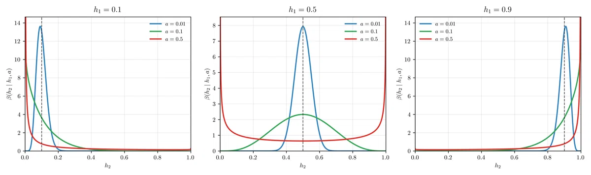
Figure 6 shows the beta distribution for $h_1=0.1,\, 0.5,\, 0.9$ from left to right. Each graph draws the cases $a=0.01,\, 0.1,\, 0.5$ in blue, green, and red respectively. When the value of the parameter $a$ is small (blue curve), the variance is small, and the distribution develops mainly around the first-street hand strength $h_1$. On the other hand, when the value of $a$ is large (red curve), the variance is large, creating a situation where the hand develops in a polarized fashion near the two ends, 0 and 1. While the average hand strength does not change across streets, the variance of hand strength (= polarizability) is tuned according to $a$.

Below, we present the Nash equilibrium for several values of $a$. Note that since the Nash equilibrium of this model is difficult to obtain analytically by hand, we discretize the continuous range on $[0, 1]$ and compute it numerically using a custom toy-model solver based on CFR. The discretization divides the interval $[0, 1]$ into 50 bins, and the exploitability is kept within an accuracy of less than 0.1% of the pot.

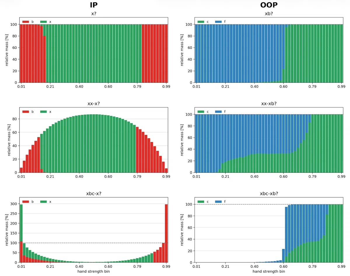
First, as a check on the computation, let us look at the result for $a=10^{-4}$ [Figure 7]. In each bar graph in Figure 7, the horizontal axis is the binned hand strength, and the vertical axis represents the relative amount when the amount in each bin on the first street is taken as 100%.

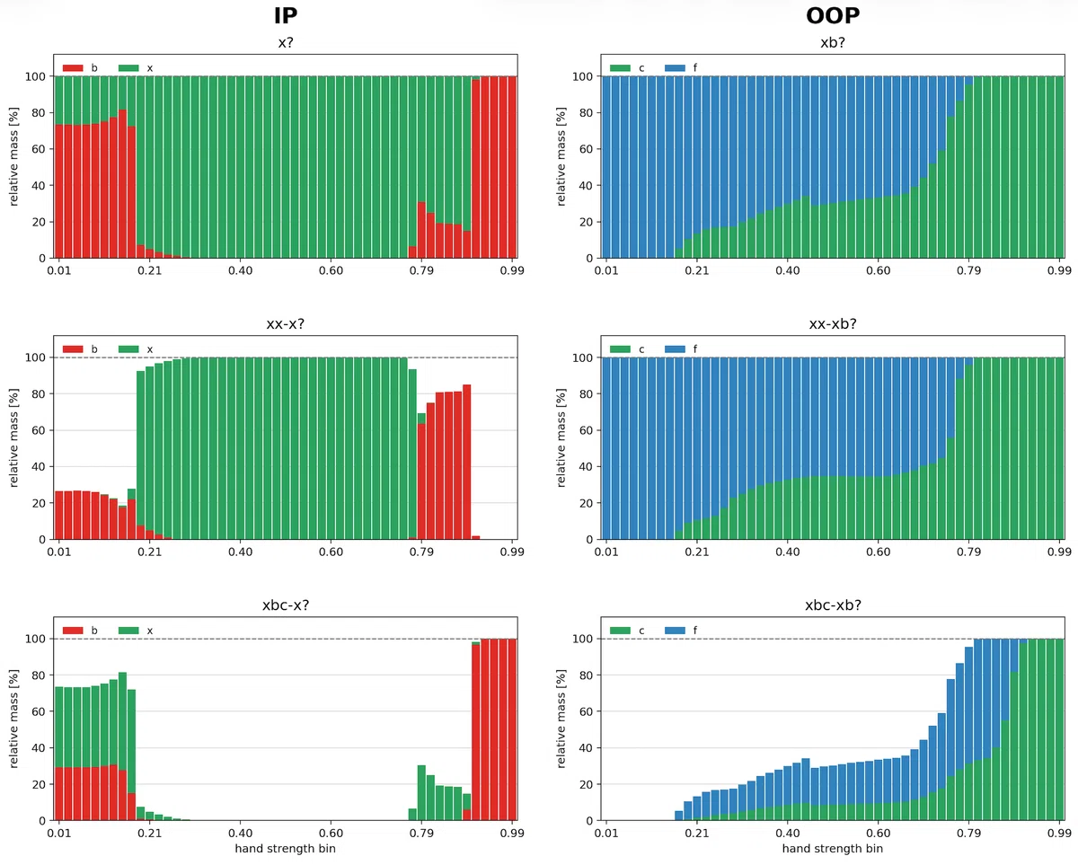
Looking at Figure 7, we see that polarized bets are made across the two streets. However, at the x? node and the xbc-x? node, the bluff bets or value bets do not form a threshold strategy. This is because this model's Nash equilibrium has degrees of freedom. For example, at the xbc-x? node, since there are no weak hands in OOP's xbc range, IP may adopt any hand with 0 EQ as a bluff on the second street.

For a small value such as $a=10^{-4}$, IP's hand strength barely changes across streets. For the completely static model in the case $a\to 0$, when using a continuous (non-discretized) range, (one of) the Nash equilibria can be found by hand. Based on that, the EVs of OOP and IP are $\frac{148}{363}\simeq 0.4077$ and $\frac{215}{363}\simeq 0.5923$ respectively. The EVs of OOP and IP obtained from the solver for $a=10^{-4}$ are 0.4106 and 0.5894 respectively. Since discretizing into 50 bins could reasonably cause about a 2% deviation of the pot from the continuous case, the solver is most likely working correctly. Let us trust the solver's results and proceed.

Figures 8 and 9 show the results for $a=0.1$ and $a=0.5$ respectively.

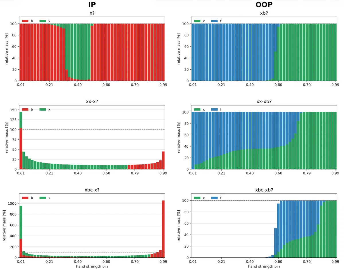
As we increase $a$, reflecting the fact that IP can polarize more strongly on the second street, we see that even marginal hands can carry a bet frequency.

Now let us see how the EV changes as we vary $a$ [Figure 10]. Figure 10 plots how the EVs of OOP and IP change as $a$ is varied. As IP's polarizability rises, it becomes possible to polarize more on the later street, and IP's EV rises monotonically.

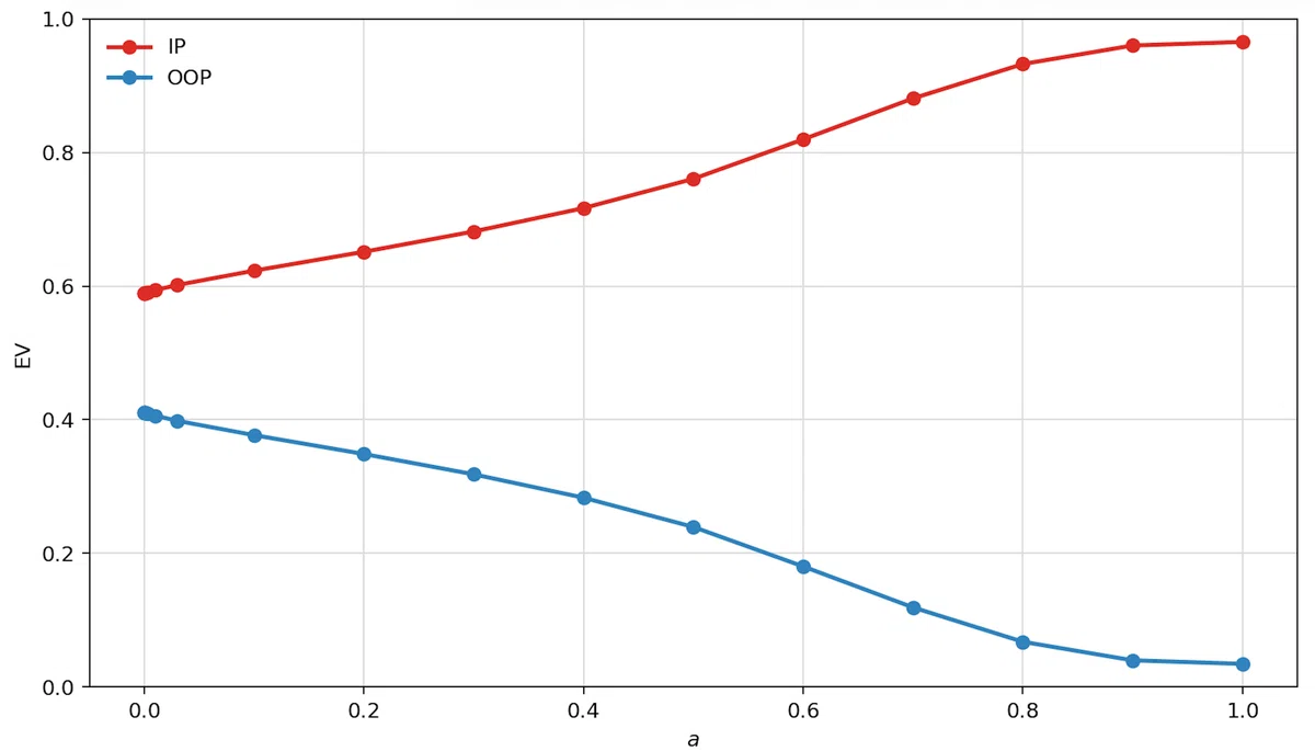
Polarizability EV is difficult to define clearly in a form directly applicable to real poker. As a rough concept, polarizability EV should be something like "the EV lost when the strengths of all hands in both ranges are assumed not to change on subsequent streets." Based on this, at least in this model, we may define the difference from the EV in the case $a=0$ as the polarizability EV.

From Concrete Spots

In real poker, polarizability includes two kinds of change in polarization, in the following sense. Picturing the progression from turn to river, the first is the change in range polarization when focusing on a single river card, and the second is the change in the sense of which river card is selected.

In the beta-[0, 1] model above, there is no new information common to both players (= river card) at the point the street advances; we modeled it simply as IP's range changing in strength (in polarization) hand by hand. In real poker, when a river card is fixed, the hand strength (EQ) is fixed, so the situation differs from the model. However, if we group together draws in a similar EQ band on the turn as a single hand group, the situation is similar. That is, for a single river card, that draw group forms a distribution in which some draws complete and advance to strong hands, some hit the river card and have marginal EQ, and the rest make no progress at all and become trash hands. The distribution differs by river card, but in the beta-[0, 1] model we forget such per-river-card details and instead describe an "average" river card.

Now, in the beta-[0, 1] model discussed in the previous chapter, we used the value $a$ as the parameter tuning a range's polarizability. Through $a$, a hand $h_1$ had a variance of $ah_1(1-h_1)$ in its strength on the subsequent street. What is the value of this $a$ in real poker?

As an example, let us look at the following spot. Figure 11 is a BTN vs. BB SRP on the 9s7s4h-Jd board that has proceeded xx-x. Having gone through a flop check-around and a turn OOP check, the two players' EQ distributions are relatively close.

Here, we trace the change in the EQ distribution for the case where the river card 8h falls and completes a GSSD. Figure 12 shows how each hand in BTN's xx-x? range changes in EQ against BB's xx-x range depending on the river card. The black diamond marks represent the average river EQ for the hand group within each 10% turn EQ bin, and the error bars represent the standard deviation of that EQ.

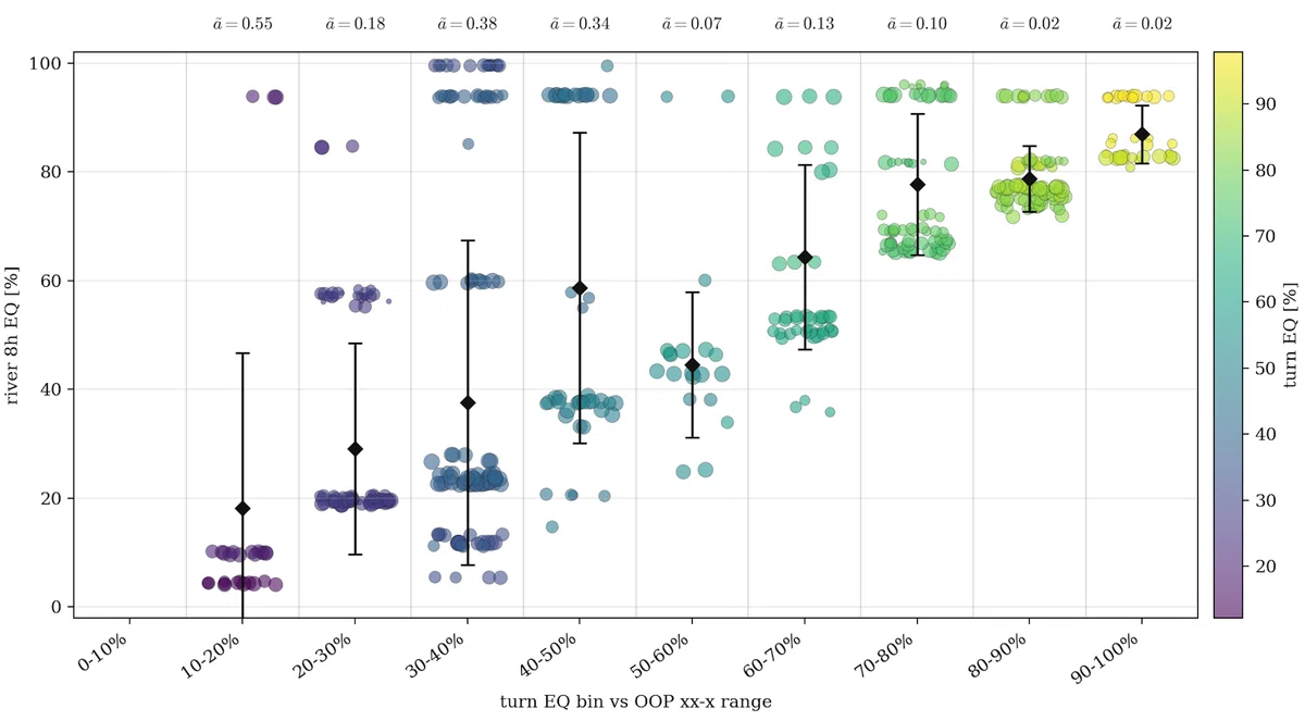
For each turn EQ bin, we compute the polarizability index $\tilde{a}$ against the beta-[0, 1] model as follows. Letting the mean EQ within a bin on the river be $h$ and the standard deviation be $\sigma$,

$$ \begin{align*} \tilde{a} = \frac{\sigma^2}{h(1-h)} \end{align*} $$

is used. In the beta-[0, 1] model, for a hand of strength $h_1$, the variance of its strength on the subsequent street satisfied

$$ \begin{align*} \sigma^2 = a\,h_1(1-h_1) \end{align*} $$

using the polarizability parameter $a$. In real poker, this amounts to estimating the polarizability parameter in reverse from the mean and variance of the hand EQ (on the river). Figure 12 records the value of $\tilde{a}$ computed for each turn EQ bin. $\tilde{a}$ varies considerably by bin. The low-EQ hand group has relatively large $\tilde{a}$ around 0.1–0.5, while the high-EQ hand group has relatively small $\tilde{a}$ of 0.1 or less.

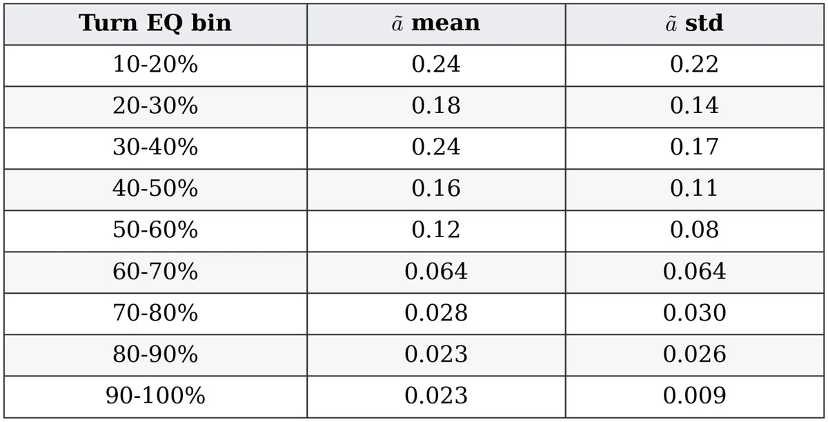
Taking the average of $\tilde{a}$ over all river cards gives Figure 13. There is a large difference in the value of $\tilde{a}$ not only by dependence on the turn EQ bin but also by river card.

The river card 8h we just looked at develops many draw cards, so $\tilde{a}$ was large for the low-EQ hand group; but for river cards that pair the board such as J or 9, or river cards almost unrelated to either range such as 2c, $\tilde{a}$ becomes as small as the order of $10^{-2}$ for many EQ bins. Taking the average over all these river cards, the low-EQ hand group appears to take values around 0.2 and the high-EQ hand group around 0.02.

Note: Because we partition the turn EQ into bins, there is inherently some EQ variance within each EQ bin; assuming hands are uniformly distributed within a bin, a $\tilde{a}$ of about 0.005 (depending on the EQ bin) naturally arises.

We introduced (range) polarizability as a concept indicating how much range polarization will polarize on subsequent streets; but looking at the polarizability per hand (group) as above, you will notice that it resembles the concepts of EQ robustness/vulnerability.

A hand's robust EQ component refers to (although no rigorous definition exists) the EQ component that does not decrease when the opponent's range changes. Put very plainly, for weak hands it indicates the possibility of being promoted, as a draw, to a nuts-class hand, and for strong hands it indicates how unlikely they are to be outdrawn by weak hands. In other words, it corresponds to the second of the two kinds of change in polarization explained at the beginning of this section: "the change in the sense of which river card is selected." Since polarizability also includes "the change in range polarization when focusing on a single river card," it is a somewhat broader term.

Summary

In this article, we have reconfirmed and formalized what factors generate EV in poker. From the half-street situation, equity EV and polarization EV emerged as basic sources of EV. These are EVs arising from range EQ and range polarization, respectively. Furthermore, from the full-street situation, position EV naturally appeared. This was the EV arising from the inferiority/superiority of OOP/IP position. And considering the 2-street situation, we found that the factor of how much the first street's range polarization polarizes on the second street increases or decreases EV. We called this the polarizability EV in this article.

How this polarizability EV arises can be seen concretely by considering the beta-[0, 1] model. The beta-[0, 1] model is a model that allows polarizability to be tuned with a single parameter $a$, and we estimated this polarizability parameter per hand group from concrete spots.

We also confirmed that the concept of polarizability encompasses the concept of EQ robustness/vulnerability. Robustness/vulnerability had not previously been defined as a clearly quantified quantity. So this time, we presented a method for computing a polarizability index from EQ. We hope it will be useful as a quantity that characterizes properties of ranges and hand groups that cannot be described by EQ alone, for implementation in solvers, analysis of toy models, and the like.

Closing

Thank you for reading this far. If you would like to study strategies like the one in this article more systematically, please be sure to check out the other articles on Seeker Start. From the basics of the rules to intermediate and advanced strategy, we explain everything clearly along a step-by-step roadmap. Let's build strong, theory-based poker together.