A Theoretical Understanding of Optimal River Bet Sizing

Author: Sigma (Twitter: @sigm_4)

What This Article Covers

• We deepen our theoretical understanding of how to choose the optimal bet size on the river, through toy models.

• As a basic model for discussing optimal bet size, we take up the half-street AKQJ model and confirm that when the opponent holds a nut advantage, the bet size is kept finite.

• We understand, through the full-street AKQJ model, why small bets are not standard for IP on the river.

• We understand, through the 2-size half-street AKQJT model, the situations in which preparing multiple bet sizes can raise EV, and we grasp the practical situations in which a small bet from IP on the river can be chosen, as well as the spots where using multiple sizes is typically recommended.

Fundamentals

Review: The AKQ Model

Let us begin by reviewing the AKQ model. Normally, the most basic AKQ model for beginners fixes the bet size at 1 relative to a pot size of 1. This time, in order to focus on the optimal bet size, let us instead treat the bet size not as 1 but as an arbitrarily fixed value ${b}$. The AKQ model was the following model.

Half-street AKQ model

- OOP player: Holds K.
- IP player: Holds A or Q with equal probability.
- OOP is forced to check, and only IP can bet (or check) (= half-street).
- Against the opponent's bet, the options are call or fold; raising is not allowed.
- The pot size is 1, and the bet size is fixed at ${b(>0)}$.
- When OOP calls or IP checks, a showdown occurs, and the player with the higher-ranking card wins the current pot.

The Nash equilibrium of the AKQ model is: IP always bets A, and bets Q with frequency ${\alpha(b) = \frac{b}{1+b}}$ and checks it with frequency ${1-\alpha(b)}$. Against this bet, OOP calls K with frequency ${1-\alpha(b)}$ and folds it with frequency ${\alpha(b)}$. Illustrated, this looks like Figure 1.

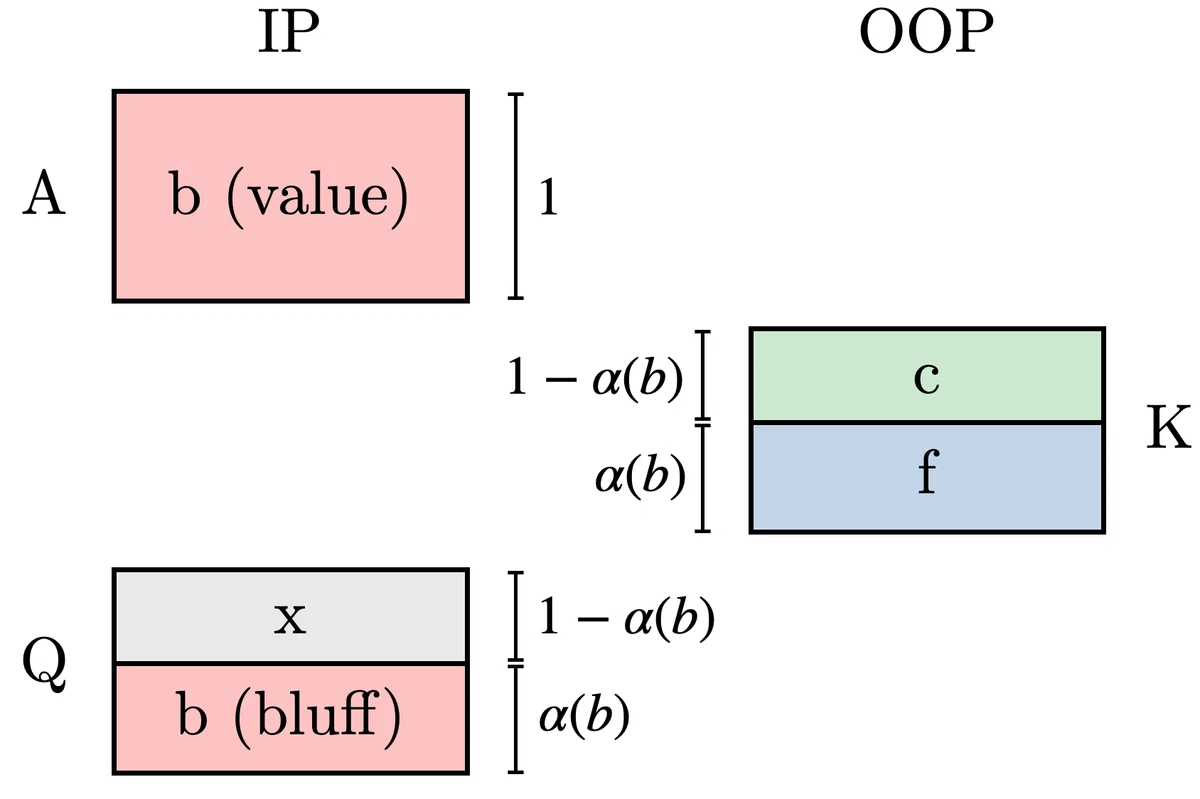
A minor note: usually the AKQ model that allows only a pot bet is introduced as a full-street game in which both OOP and IP have the right to bet. In that case, since OOP holding K simply checks, there is little difference from the half-street case. The reason we deliberately write it as half-street here is that we set the bet size to an arbitrary value ${b}$. In fact, (as long as raising is forbidden) when ${b}$ is small, a Nash equilibrium can arise in which OOP always bets. Interested readers may want to think about why.

In the Nash equilibrium of Figure 1, the EVs of OOP and IP are, respectively,

$$ \begin{align*} \mathrm{EV}_{\mathrm{OOP}}(b) &= \frac{1}{2}(1-\alpha(b)) \quad\quad (1) \\ \mathrm{EV}_{\mathrm{IP}}(b) &= \frac{1}{2}(1+\alpha(b)) \quad\quad (2) \end{align*} $$

as obtained above. This is easy to understand as follows. When IP bets, it can reduce OOP's EV to 0 (making K indifferent between call and fold), so IP obtains an EV equal to (pot size) × (bet frequency). Conversely, when OOP faces a bet from IP its EV is reduced to 0, so OOP obtains EV only to the extent that IP checks back.

So in this AKQ model, what bet size is optimal for IP to use? The answer is simple: using as large a bet size as possible is optimal. Formally, we just need to find the ${b}$ that maximizes ${\mathrm{EV}_{\mathrm{IP}}(b)}$. Looking at equation (2), ${\mathrm{EV}_{\mathrm{IP}}(b)}$ is an increasing function of ${b}$, so the larger we make ${b}$, the more IP can raise its EV.

We need not rely on formulas; it can be understood intuitively as follows. As stated above, IP's EV is determined solely by its bet frequency. The higher the bet frequency, the higher the EV, and since A is always bet, the point is simply to raise the bluff frequency. And to raise the bluff frequency, you raise the bet size.

We did not include the concept of stack (SPR) in the model's definition, but if there were a finite stack, all in would be the optimal bet size. To put it as a slogan: "For a fully polarized bet range, you want to make the bet size as large as possible."

A Basic Model for Discussing Optimal Bet Size: The Half-Street AKQJ Model

Now, in the AKQ model the result was that all in is chosen as the optimal bet size. How robust is the conclusion that "if you have a polarized bet range, go all in"? To investigate, let us consider the following AKQJ model.

Half-street AKQJ model

- OOP player: Holds A or Q with proportions ${p}$ and ${1-p}$, respectively, where ${0 \leq p \leq 1}$.
- IP player: Holds K or J with equal probability.
- OOP is forced to check, and only IP can bet (or check) (= half-street).
- Against the opponent's bet, the options are call or fold; raising is not allowed.
- The pot size is 1, and the bet size is fixed at ${b(>0)}$.
- When OOP calls or IP checks, a showdown occurs, and the player with the higher-ranking card wins the current pot.

This model lets us tune OOP's range with the parameter ${p}$. When ${p=0}$ it is equivalent to the AKQ model, so we see that this AKQJ model is a natural extension of the AKQ model. Here too we consider a half-street game with the bet size fixed at an arbitrary value ${b}$.

What is the Nash equilibrium of this model? First, as an extreme case, at ${p=0}$ it is equivalent to the AKQ model as stated above, and IP holding K or J adopts a betting strategy. In the opposite limit ${p=1}$, OOP holds only A, so IP has no recourse but to check its entire range. In other words, in this model, when ${p}$ is small IP can bet so as to squeeze Q between K and J, and as ${p}$ grows larger the chance of paying off A increases so IP can no longer bet—the behavior switches over.

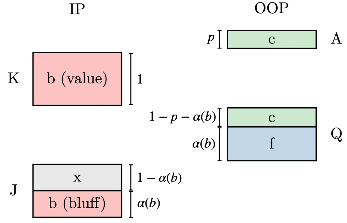
More concretely, the Nash equilibrium changes depending on the relationship between ${p}$ and ${b}$, but here let us focus on the side where ${p}$ is small. If ${p}$ is sufficiently small, IP always bets K, and bets J with frequency ${\alpha(b)}$ and checks it with frequency ${1-\alpha(b)}$. Against this bet, OOP always calls A, calls Q with frequency ${1-\frac{\alpha}{1-p}}$, and folds it with frequency ${\frac{\alpha}{1-p}}$. Figure 2 illustrates this.

The EVs of OOP and IP in this case are, respectively,

$$ \begin{align*} \mathrm{EV}_{\mathrm{OOP}}(b) &= 1-\frac{1}{2}(1+\alpha(b))(1-(1+b)p) \quad\quad (3) \\ \mathrm{EV}_{\mathrm{IP}}(b) &= \frac{1}{2}(1+\alpha(b))(1-(1+b)p) \quad\quad (4) \end{align*} $$

Equation (4) can be derived easily. Since IP obtains no EV when it checks, it can obtain EV only when it bets. When IP bets, if OOP holds Q then IP can reduce OOP's EV to 0 (= IP captures the pot of 1), so it obtains an EV equal to the bet frequency ${\frac{1}{2}(1+\alpha)}$. On the other hand, when OOP holds A, IP pays off the bet amount ${b}$. Multiplying by the probabilities that OOP holds Q and A respectively and summing gives equation (4).

So what is the bet size that maximizes IP's EV? As in the AKQ model we would like to raise the bet size to raise the bet frequency, but at the same time the amount paid off to A also grows larger, so it seems we cannot just keep raising the bet size indefinitely. And indeed, the optimal bet size turns out to be a finite value. Omitting the derivation,

$$ \begin{align*} b = \frac{1-\sqrt{2p}}{\sqrt{2p}} \quad\quad (5) \end{align*} $$

is the bet size that maximizes EV. The specific value is not so important here, but the important fact is that when the KJ side's opponent holds hands stronger than its own value hands, making the bet size infinitely large is no longer optimal. Building on the form of this model, let us proceed to the applications.

Applications

As applications, we treat two river-related topics. The first discusses why GTO strategy does not choose small bet sizes from IP on the river; the second discusses when using multiple bet sizes raises EV.

Why IP Doesn't Use Small Bets on the River: The Full-Street AKQJ Model

Many readers have probably heard the point that using a small bet size as IP on the river is not "standard." Indeed, in GTO strategy, bet sizes like 10%–40% are rarely used from IP in river spots. Let us look at some concrete examples.

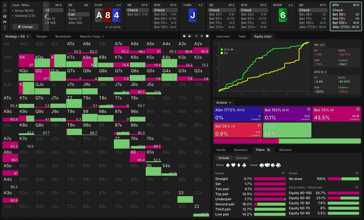
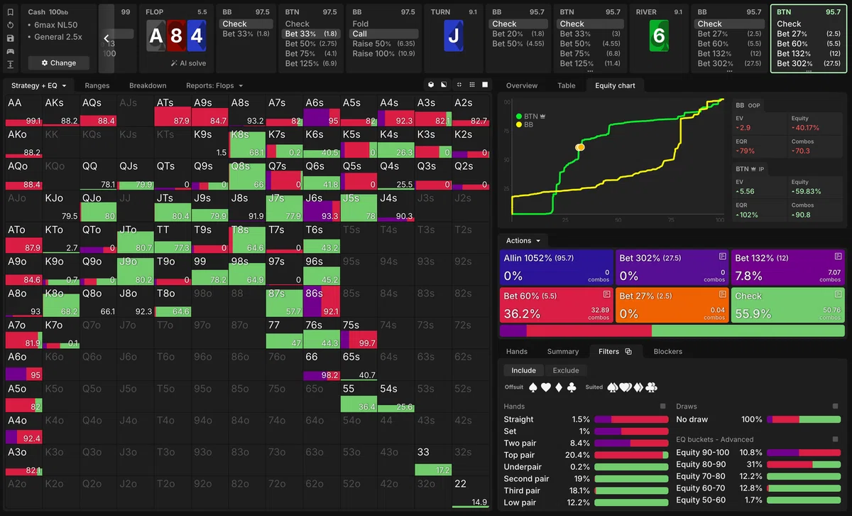
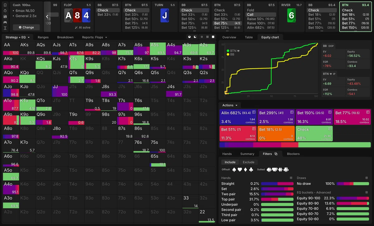
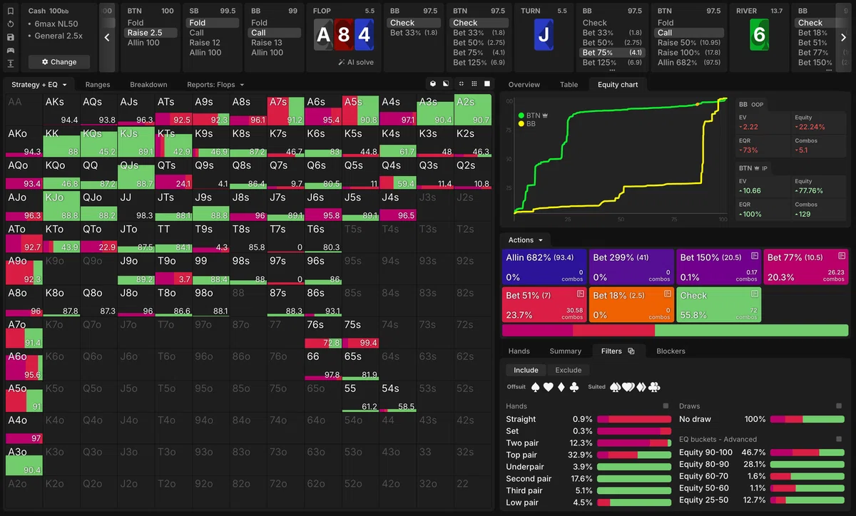
Figures 3–6 show BTN's local river strategy for four different play lines in a BTN vs. BB SRP on As8h4d-Jd-6c. Hereafter, unless otherwise noted, solutions are based on GTO Wizard, 6max Cash, 100bb, NL50, 2.5x-GTO. Figure 3 corresponds to xx-xx-x?, Figure 4 to xb 33%c-xx-x?, Figure 5 to xx-xb 75%c-x?, and Figure 6 to xx-b 75%c-x?.

In every case we see that small bet sizes are (almost) never used. At least from these four patterns, the smallest bet size used with (sufficient) frequency appears to be 51%. Looking at the EQ graphs, even though the EQ distribution differs greatly depending on the line taken, IP stubbornly avoids small bet sizes and adopts only sizes ranging from 51% up to the 682% all in.

Why does this happen? If it is a universal phenomenon, it should be understandable from a simple model.

At the point of entering the river, there are broadly two patterns to consider.
(1) The case where IP has the nut advantage.
(2) The case where OOP has the nut advantage.

Abstracting (1) into a model, it is a situation where OOP holds K or J and IP holds A or Q. In this case, against OOP's check, IP bets so as to squeeze K between A and Q—and this is exactly the same as the AKQ model, a situation where the larger the bet size, the more EV can be captured.

Note: When IP holds A above a certain proportion, OOP is forced to check. Against that check, IP goes all in with A and Q. When IP's proportion of A is small, the equilibrium becomes one where OOP's KJ side bets and the AQ side raises against it. Since OOP uses all of its K in betting, against OOP's check IP forms a "meaningless" bet range (a threat with no indifference target).

As in the xx-xb 75%c-x? case of Figure 5, the situation where BTN bets the turn and enters the river with a polarized range is a typical example of (1). Indeed, looking at Figure 5, we see that even huge bet sizes such as the 682% all in are used.

What about case (2)? As we saw in the half-street AKQJ model in the Fundamentals, when OOP has the nut advantage, a constraint should arise whereby IP cannot make its bet size large. Intuitively, it seems small sizes ought to be permissible. To verify this, let us build a concrete model. A naive model would be the full-street AKQJ model where OOP holds A or Q and IP holds K or J.

Full-street AKQJ model

- OOP player: Holds A or Q with equal probability.
- IP player: Holds K or J with equal probability.
- OOP can bet (or check) first, and if OOP checks, IP can also bet (or check) (= full-street).
- Against the opponent's bet (or raise), the options are fold, call, or raise.
- The pot size is 1, the stack is ${S}$, and any bet size and raise size can be chosen.
- When one player's bet is called by the other, or when both players check, a showdown occurs, and the player with the higher-ranking card wins the current pot.

This model is brought closer to real poker by allowing raises, and we find the Nash equilibrium under the assumption that any bet size and raise size can be chosen.

Note: Rather than using a fixed bet (raise) size, the model is defined as a game in which any bet (raise) size is allowed.

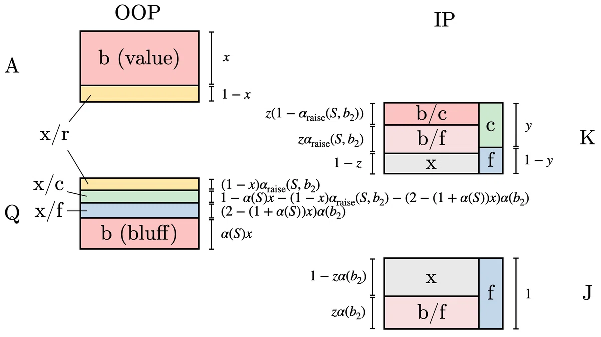
Keeping in mind that both OOP's optimal bet size and raise size are all in, we set IP's bet size to ${b}$ and assume the Nash equilibrium has the form of Figure 7. We let OOP's bet frequency with A be ${x}$, IP's call frequency with K against OOP's bet be ${y}$, and IP's bet frequency with K after OOP's check be ${z}$.

Under this, we set up equations so that each action is indifferent. In what follows we use alpha defined as follows.

$$ \begin{align*} \alpha(S) &= \frac{S}{1+S}, \quad\quad (6) \\ \alpha(b) &= \frac{b}{1+b}, \quad\quad (7) \\ \alpha_{\mathrm{raise}}(S, b) &= \frac{\alpha(S)-\alpha(b)}{1-\alpha(S)\alpha(b)}. \quad\quad (8) \end{align*} $$

Equation (6) is the alpha for OOP's all in, equation (7) is the alpha for IP's bet, and equation (8) is the alpha for OOP's all-in raise against IP's bet.

We take up only the minimum portion of the calculation needed for the discussion of bet-size optimization. The remaining details are described later. First, from the fact that the EVs of betting and checking K for IP are equal,

$$ \begin{align*} x = \frac{(1+\alpha(b))\alpha_{\mathrm{raise}}(S, b) + 2\alpha^2(b)}{(1+\alpha(b))\alpha_{\mathrm{raise}}(S, b) + \alpha(b)(1-\alpha(S)+(1+\alpha(S))\alpha(b))} \quad\quad (9) \end{align*} $$

is obtained.

Next we find the EV each player captures. Using the fact that IP can obtain EV only after OOP checks, and that both K and J are indifferent between bet and check,

$$ \begin{align*} \mathrm{EV}_{\mathrm{OOP}} &= 1-\frac{1-\alpha_S x}{4}, \quad\quad (10) \\ \mathrm{EV}_{\mathrm{IP}} &= \frac{1-\alpha_S x}{4} \quad\quad (11) \end{align*} $$

is derived. Since ${\mathrm{EV}_{\mathrm{IP}}}$ is monotonically decreasing in ${x}$, setting the bet size ${b}$ so as to minimize ${x}$ creates the Nash equilibrium of this game.

We omit the specific calculation, but differentiating ${x}$ with respect to ${\alpha(b)}$ and finding the bet size ${b^*}$ that gives the minimum,

$$ \begin{align*} \alpha(b^*) &= \frac{1}{1+2\alpha(S)}, \quad\quad (12) \\ b^* &= \frac{1+S}{2S} \quad\quad (13) \end{align*} $$

is obtained.

${b^*}$ is a decreasing function of the SPR ${S}$, and

$$ \begin{align*} b^* > \frac{1}{2} \quad\quad (14) \end{align*} $$

holds. In other words, this suggests that even when OOP has the nut advantage upon entering the river and there is a factor that could lower IP's bet size, IP's optimal bet size does not fall below 50% of the pot.

Note: As described later, for ${S \geq 1}$ the Nash equilibrium with this bet size ${b^*}$ holds. Also, for ${S \leq 1}$, IP's optimal bet size is all in.

Spelling out the structure of the Nash equilibrium when IP uses the bet size ${b^*}$: First, OOP wants to use A and Q to go all in, squeezing K. But if it uses up all of its A, it then faces a bet from IP squeezing Q between K and J. If no A is left at all, this IP bet is best made all in, and the loss is large. To prevent this, OOP tries to keep some of its A appropriately in its check range to counter IP's bet. On the other hand, if OOP keeps too much A in its check range it loses the EV it would have obtained by going all in, so it must mix check and bet "appropriately." This "appropriateness" is tuned so that IP's K is indifferent between bet and check.

As we saw in the Fundamentals, after OOP checks, IP has no nut advantage so it cannot make its bet size infinitely large, and it chooses an appropriate finite bet size. If IP's bet size is too large, OOP can exploit by keeping all of its A in the check range, and conversely if IP's bet size is too small, OOP can exploit by using up all of its A on the all in. As a result of this tension, a bet size around (or above) 50% of the pot is what gets chosen.

Let us return to practical spots. As in Figure 3 or Figure 4 where BTN checks back the turn and gives up its high-EQ hands, or as in Figure 6 where BB probe bets the turn and polarizes, the situation corresponds to case (2) where OOP has the nut advantage upon entering the river. In this case, by the argument above, upon facing OOP's river check IP chooses a bet size larger than 50%.

From the above, we see that whether or not OOP has the nut advantage, IP's bet size never becomes too small.

######

Below we verify the Nash equilibrium, but since it is a detailed discussion, readers who are not interested in the calculation details may skip it.

From the fact that the EVs of betting and checking Q for OOP are equal,

$$ \begin{align*} y = (1-\alpha(S))(1+\alpha(b)z), \quad\quad (15) \end{align*} $$

and from the fact that the EVs of betting and checking A for OOP are equal,

$$ \begin{align*} y = \frac{1+\alpha(b)}{1+\alpha_{\mathrm{raise}}(S,b)}z, \quad\quad (16) \end{align*} $$

can be derived. Then from equations (15) and (16),

$$ \begin{align*} y &= \frac{1-\alpha^2(S)}{1+\alpha^2(S)}, \quad\quad (17) \\ z &= \frac{\alpha(S)(1-\alpha(S))(1+2\alpha(S))}{1+\alpha^2(S)} \quad\quad (18) \end{align*} $$

is obtained. Also, using equations (9) and (12),

$$ \begin{align*} x = 1-\frac{1-\alpha(S)}{\alpha(S)(3+4\alpha(S))} \quad\quad (19) \end{align*} $$

follows. Therefore, ${0 < x, y, z < 1}$ holds identically.

Solving ${b^*\leq S}$ for IP's optimal bet size ${b^*}$,

$$ \begin{align*} S \geq 1 \quad\quad (20) \end{align*} $$

is obtained.

Computing OOP's x/c and x/f frequencies with Q gives ${\frac{4\alpha(S)(1-\alpha(S))}{3+4\alpha(S)}}$ and ${\frac{(1-\alpha(S))(1+2\alpha(S))}{\alpha(S)(3+4\alpha(S))}}$, respectively; these always take values between 0 and 1 for SPR ≥ 1, and the assumed Nash equilibrium holds.

Therefore, when the SPR is 1 or greater, IP chooses ${b^* (\leq S)}$ as its bet size, and when the SPR is less than 1, it goes all in.

When Using Multiple Bet Sizes Is Beneficial: The 2-Size Half-Street AKQJT Model

As the second application, let us consider from a model the situations where using multiple bet sizes is beneficial. The toy models we commonly see basically allow either a single fixed bet size, or, as in the first application, an arbitrary single size. This time, let us look at a model that can prepare two variable bet sizes. With this we investigate in what situations increasing the bet sizes can raise EV.

Considering two sizes in a full-street model is too difficult, so let us think in half-street. First, in the minimal-range AKQ model, the AQ side just wants to make the bet size large, so increasing the bet-size options is meaningless. As for the AKQJ model, both the AQ side and the KJ side have an optimal bet size, so again increasing the bet-size options does not change EV. So what about adding one more card, an AKQJT model where one side holds A, Q, T and the other holds K, J?

2-size half-street AKQJT model

- OOP player: Holds K or J with proportions ${p}$ and ${1-p}$, respectively, where ${0<p<1}$.
- IP player: Holds A, Q, or T with probabilities ${\frac{1}{4}, \frac{1}{4}, \frac{1}{2}}$, respectively.
- OOP is forced to check, and only IP can bet (or check) (= half-street).
- Against the opponent's bet, the options are fold, call, or all-in raise.
- The pot size is 1, the stack is ${S}$, and any two bet sizes ${b_1, b_2}$ can be chosen (${b_1 \geq b_2 > 0}$).
- When either player calls or IP checks, a showdown occurs, and the player with the higher-ranking card wins the current pot.

Note: To simplify the problem, the raise size is limited to all in. Also, to avoid the complication of case splitting, the amount of T that IP holds is made twice that of A and Q.

A bet of bet size ${b_1}$ with A and T is trivially best made all in. So we assume the Nash equilibrium of this game has the form of Figure 8. We let IP's frequency of betting (going all in) at bet size ${S}$ with A be ${x}$, and OOP's call frequency with K when facing a bet of size ${b_2}$ be ${y}$.

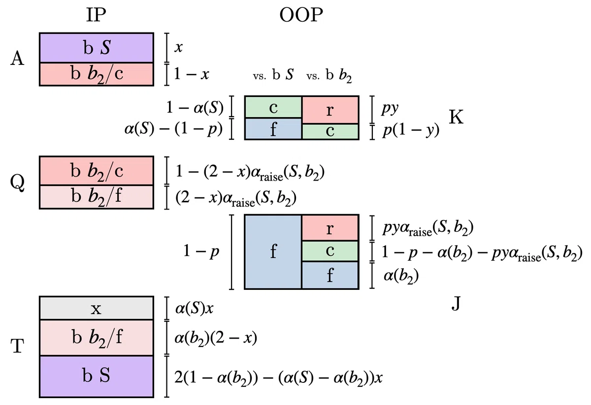
It is natural that IP uses A and T to bet (go all in) so as to squeeze IP's [opponent's] K and J. As for IP's Q, checking seems good if OOP's proportion of K is large, but if K is somewhat scarce, IP can bet so as to squeeze J between Q and T. Since OOP can raise against IP's bet, to keep that raise from being extra profitable, IP includes A in the thin-value bet range with Q to form a trap range.

Again let us solve only the minimum portion needed for the discussion. First, from the fact that the EVs of raising and calling K for OOP are equal,

$$ \begin{align*} x = \frac{2\alpha_{\mathrm{raise}}(S,b_2)}{1+\alpha_{\mathrm{raise}}(S,b_2)} \quad\quad (21) \end{align*} $$

is obtained. Noting that OOP's EV arises from the fact that OOP always captures the pot when IP checks, and from the case where OOP holds K when IP bets at size ${b_2}$,

$$ \begin{align*} \mathrm{EV}_{\mathrm{OOP}} = \frac{1}{4}(2+p-2\alpha(b_2)(1-p(1+b_2))-(\alpha(S)-\alpha(b_2))x) \quad\quad (22) \end{align*} $$

can be derived. Substituting equation (21) into equation (22) and differentiating with respect to ${\alpha(b_2)}$, we find the bet size ${b_2=b^*}$ at which OOP's EV takes a minimum. Omitting the calculation details and stating only the result,

$$ \begin{align*} \alpha(b^*) &= 1 - \sqrt{3 - \alpha(S) - \frac{1+\alpha(S)}{\alpha(S)}(1-p)}, \quad\quad (23) \\ b^* &= \frac{1-\sqrt{3 - \alpha(S) - \frac{1+\alpha(S)}{\alpha(S)}(1-p)}}{\sqrt{3 - \alpha(S) - \frac{1+\alpha(S)}{\alpha(S)}(1-p)}} \quad\quad (24) \end{align*} $$

is obtained.

The details are given later as a supplement, but there is a condition for whether this extremum is directly the point of minimum EV, and

$$ \begin{align*} (1-\alpha(S))^2 \leq p < \frac{\alpha(S)}{2} - \frac{(1-\alpha(S))-\alpha(S)\sqrt{2(1-\alpha(S))}}{1+\alpha(S)} \quad\quad (25) \end{align*} $$

in this case the strategy ${b_2=b^*}$ above constitutes a Nash equilibrium.

If the SPR is sufficiently large, the lower bound approaches 0 and the upper bound approaches 1/2. Let us specifically look at the behavior of IP's optimal bet size by sweeping ${p}$ at ${S=10}$. Figure 9 plots ${b^*}$ as a function of ${p}$. The vertical dotted lines represent the upper and lower bounds of ${p}$ corresponding to equation (25).

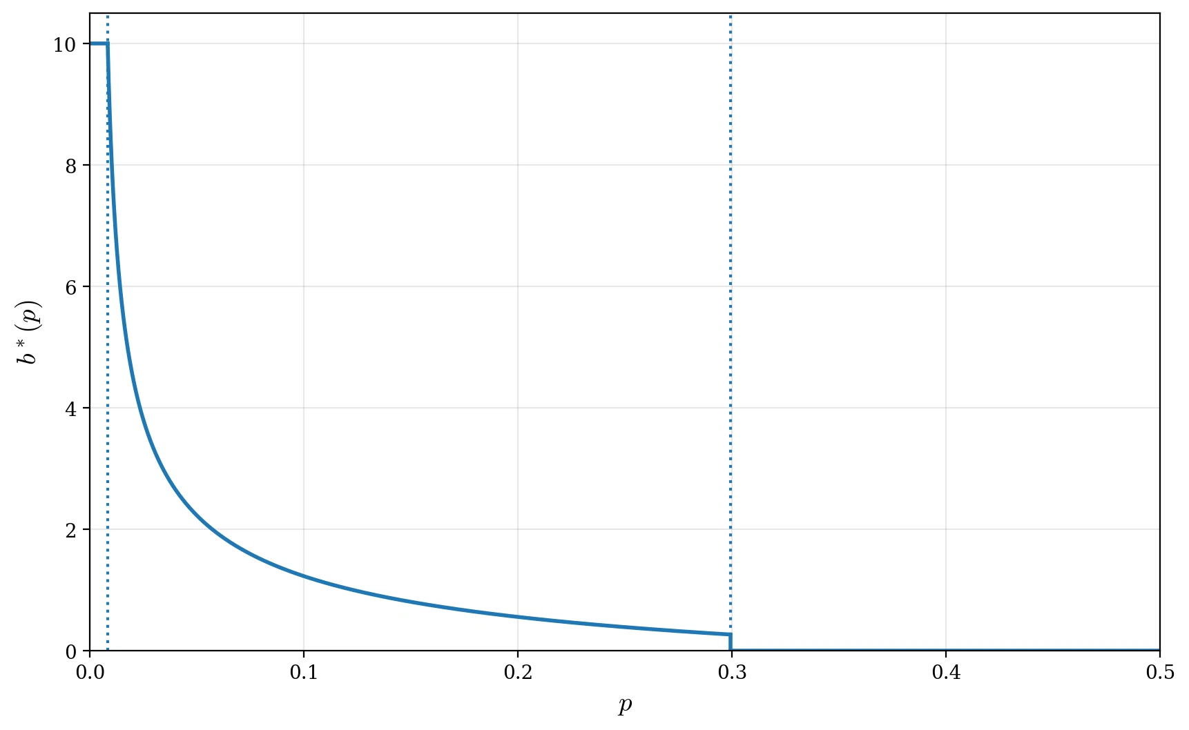
In the range of equation (25), the optimal bet size ${b^*}$ varies with ${p}$. As OOP's proportion of K increases, IP's optimal bet size with Q gradually shrinks, and eventually becomes 0 (the check EV becomes higher). This has the same structure as the optimal bet size of the KJ side in the AKQJ model of the Fundamentals.

To summarize so far: within the range satisfying equation (25) (≈ a situation where OOP's proportion of K is somewhat small and the SPR is somewhat large), it becomes beneficial for the AQT side to use two bet sizes, large and small. The structure is to squeeze OOP's K and J with the large size (all in) using A and T, mix part of the A into a trap, and then bully J with Q as the main value hand. Let us confirm that using two different sizes does indeed yield higher EV than using only one size. Organizing IP's EV in this two-size model using equations (23)–(24) in equation (22),

$$ \begin{align*} \mathrm{EV}_{\mathrm{IP}}^{(2)} = \frac{2-p+\alpha(S)}{4} + \frac{\alpha(S)}{4(1+\alpha(S))}(2\alpha^2(b^*)-(1-\alpha(S))) \quad\quad (26) \end{align*} $$

is obtained. Here we put a (2) on the shoulder to make explicit that this is the two-size strategy. We compare this against the EV in the Nash equilibrium that uses only a single optimal bet size. If OOP's proportion of K is large, IP should bet only with A and T and check Q. The optimal bet size here is all in, and IP's EV is

$$ \begin{align*} \mathrm{EV}_{\mathrm{IP}}^{(1)} = \frac{2-p+\alpha(S)}{4} \quad\quad (27) \end{align*} $$

If OOP's proportion of K is small, IP does better to also bet Q as a value hand. A simple calculation shows the optimal bet size is

$$ \begin{align*} b = \begin{cases} \frac{1-\sqrt{p}}{\sqrt{p}} & \text{if}\quad p \geq (1-\alpha(S))^2 \\ S & \text{if}\quad p \leq (1-\alpha(S))^2 \end{cases} \quad\quad (28) \end{align*} $$

Correspondingly, IP's EV in this Nash equilibrium is

$$ \begin{align*} \mathrm{EV}_{\mathrm{IP}}^{(1')} = \begin{cases} (1-\frac{\sqrt{p}}{2})^2 & \text{if}\quad p \geq (1-\alpha(S))^2 \\ \frac{1+\alpha(S)}{4}(2-\frac{p}{1-\alpha(S)}) & \text{if}\quad p \leq (1-\alpha(S))^2 \end{cases} \quad\quad (29) \end{align*} $$

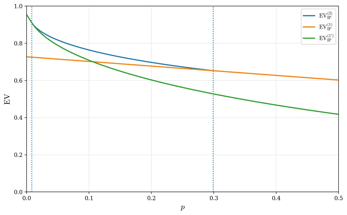
Plotting equations (26), (27), and (29) for the case ${S=10}$ gives Figure 10. The blue, yellow, and green curves depict, respectively, the behavior of IP's EV using two sizes (equation (26)), IP's EV using a single size when ${p}$ is large (equation (27)), and IP's EV using a single size when ${p}$ is small (equation (27)). The vertical dotted lines represent the upper and lower ends of the condition in equation (25). We see that within the range of ${p}$ satisfying equation (25), IP can raise its EV by adopting the two-size strategy over the one-size strategy.

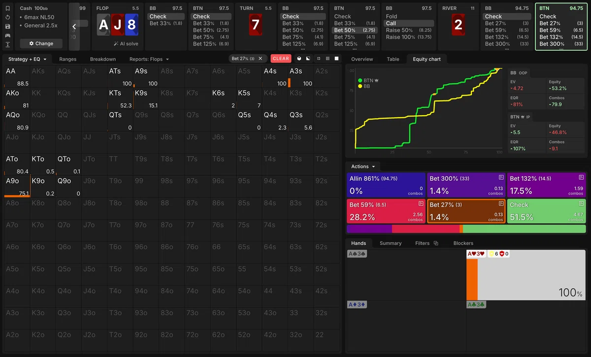
Now let us return to the topic of optimal bet size. When we allow the use of two sizes, the thin value bet with Q was formed by the cheaper bet size. Looking at Figure 9, if ${p}$ is somewhat large (at least in the case ${S=10}$), this bet size can become quite small. For example, near the boundary at ${p\simeq 0.3}$ we get ${b^*\simeq 0.27}$. In the previous section we argued that IP's optimal bet size becomes larger than 50%, but this shows that if IP's river action decision reaches a situation like this half-street AKQJT model, a small bet size can be used with some frequency in the Nash equilibrium that allows multiple sizes.

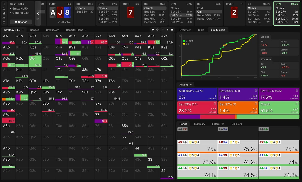
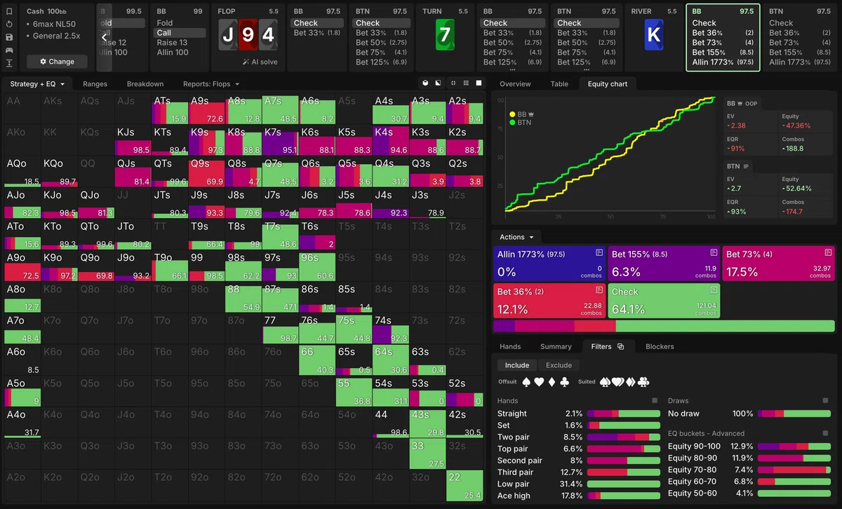
So can such a situation actually occur? Let us look at the following spot. Figure 11 is a BTN vs. BB SRP on the board AsJh8d-7h-2h that has proceeded xx-xb 50%c-x?. Here, IP's main bet sizes are 59% and 132%, but there is a slight option of a small size of 27%. Since the bet frequency viewed across the whole range is very small, at first glance it might seem like a calculation error or an artifact arising because the optimal bet size is not in the game tree—but that should not be the case. Indeed, A9o holding Ah purely chooses this bet size, with an EV difference of about 0.08 from check, the next-highest-EV action (the error at this infoset is typically about 0.02). Also, filtering to display b 27% [Figure 12], we see that besides Ah9x, flushes such as Ah3h and Ah9h are in the trap range, and some K-high and Q-high hands (such as K9o) are adopted as bluffs. This closely resembles the AKQJT model's structure of placing Q as the main value hand and trapping some A.

Let us think, based on the AKQJT model, about what conditions create such a small bet-size option for IP on the river. First, for Q to be able to bet, there must be many hands in OOP's range corresponding to the J that it makes indifferent. Furthermore, if OOP's proportion of K is too large, Q can no longer bet, so K must be below a certain amount. According to the AKQJT model for ${S=10}$, this criterion is roughly ${p\lesssim 0.3}$. Conversely, if OOP's proportion of K is too small, then Q's optimal bet size rises, so the small size is no longer chosen. In other words, if OOP consumes its K on the river bet, this is no longer realized. Since this happens when IP's proportion of A is small, it is also important that IP has a sufficient amount of A upon entering the river. To summarize: a situation where IP has a fair amount of top range (= A) upon entering the river, OOP cannot consume its value hands (= K) and checks, and there exists in OOP a target (= J) for IP to fire a thin value bet at. As in the earlier spot, in a situation where IP fires a delayed CB on the turn and polarizes, and then the river completes a flush so that OOP is replenished with high-EQ hands, this condition may be satisfiable. If a card that substantially replenishes OOP's top range falls on the river (such as Js), IP can no longer fire a thin value bet; and if a rag that does not increase OOP's high-EQ hands falls (such as 2s), IP can make its thin value hand's bet size larger. Whether a small thin value bet from IP is possible is quite delicate.

This time, partly because the model is half-street, we focused especially on IP's river bet size. However, the kind of local strategy seen in the 2-size AKQJT model—using larger and smaller bet sizes according to the strength of the value hand—also occurs for OOP on the river. A particularly typical case is the xx-xx-? infoset, where OOP's and IP's EQ distributions are close to each other. Here OOP can use a wide range of sizes from large to small to raise EV. As a model, the well-known [0, 1] model describes this well. OOP's basic bet strategy is the same as in the AKQJT model: it uses different bet sizes according to hand strength, while mixing its very strong hand group as a trap range not only into the large size but also into medium and small sizes.

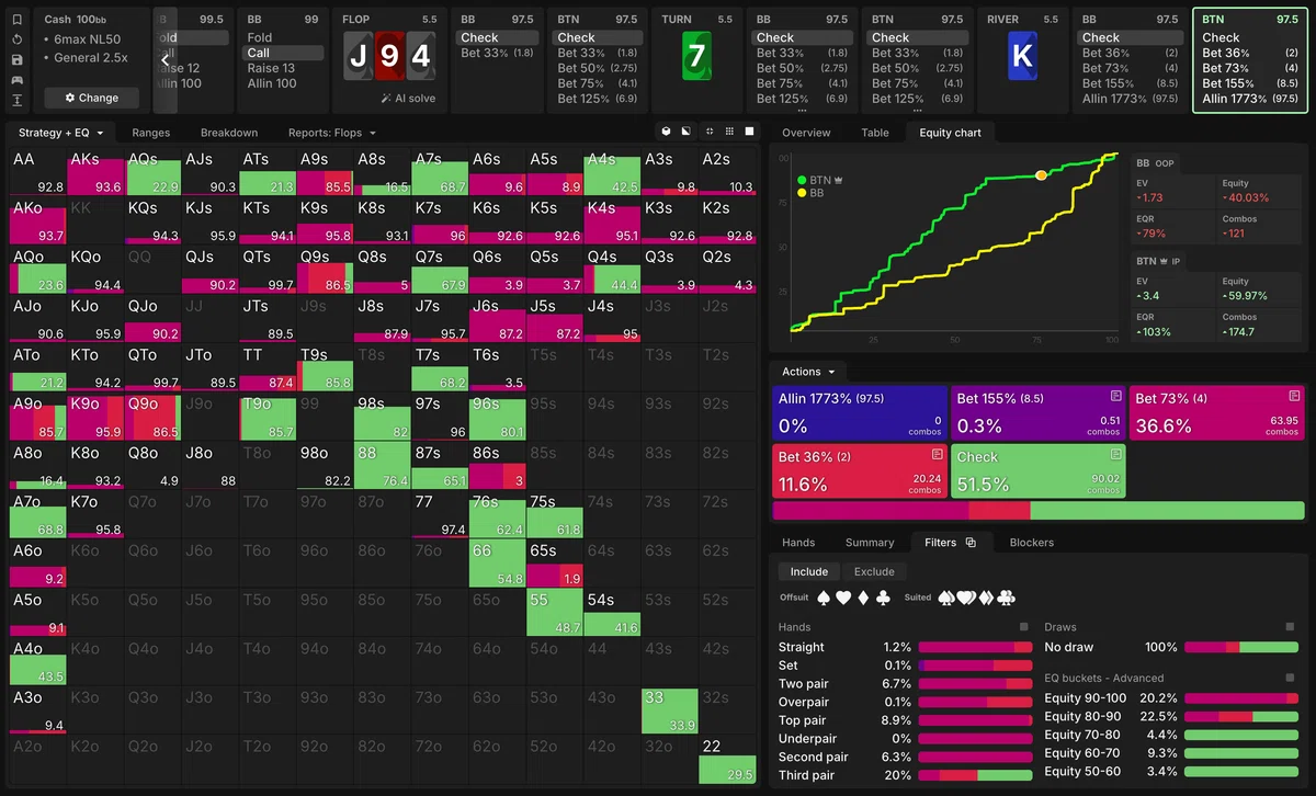
For example, as in Figure 13, in a BTN vs. BB SRP on the board Js9h4s-7c-Kd that has proceeded xx-xx-?, OOP uses all of the large, medium, and small bet sizes—155%, 73%, and 36%. 155% mainly uses two pair, 73% mainly top pair and second pair, and 36% mainly third pair, as their main value hands. For the very strong hand group of two pair and above, frequency is created not only in the large size but also in the medium and small sizes, forming a trap range. Note too that many nuttish hands such as straights and sets go to check and are trapped.

Looking at BTN's local strategy when BB checks from here [Figure 14], we see that BTN has the option of a small bet size, b 36%. However, this bet size may not necessarily be a robust result, and caution is needed. In fact, as shown in Figure 15, if we prepare finer river bet-size options such as 33%, 51%, 75%, … (details in the note), the hands that originally chose b 36% switch to using b 51% instead, and the frequency of b 33% plummets. In other words, this may be an artifact arising because the bet size around 50% that was actually desired did not exist in the default game tree.

Looking at the xx-xx-x? infoset in GTO Wizard's solutions, small bet sizes below 50% are used fairly frequently. In GTO Wizard's 100bb SRP, a size around 50% does not exist by default for IP's bet size at xx-xx-x?, so frequency can concentrate on small bet sizes that are not necessarily essential in this way. Caution is needed if you want to engage in memorizing "in this spot, this bet size is good."

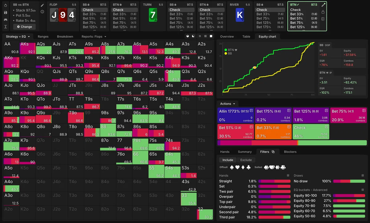
Note: Figure 15 was precisely created as follows. First, we create a solution once, specifying bet sizes of 33%, 50%, 125%, 175%, 250% on the flop/turn and 33%, 75%, 125%, 175%, all in on the river (call this solution A). Next, for this turn and river card, we nodelock all local strategies up to xx-xx-x to the local strategies contained in solution A. Here, we add 51% to the bet sizes at the xx-xx-x? infoset and obtain a fresh solution (call this solution B). The local strategy for BTN at xx-xx-x? contained in solution B is Figure 15. In other words, we are comparing the solutions of two subgames that use the same BTN range at the river xx-xx-x? infoset but have different sets of bet sizes. In solution A this local strategy has a b 33% frequency of about 6–7%, but in solution B the b 33% frequency drops to 0.7%.

######

Below we present the details of the Nash equilibrium of the AKQJT model, along with the calculation verifying that the Nash equilibrium with the optimal bet size ${b^*}$ exists when the condition of equation (25) is satisfied. Readers who wish to follow the details are welcome to read on.

First, let us find the frequency of each action in the Nash equilibrium assumed as in Figure 8. From the fact that the EVs of IP betting A at size ${b_1=S}$ and at size ${b_2}$ are equal,

$$ \begin{align*} y = \frac{1}{p}\cdot\frac{1-\alpha(S)}{1+\alpha(S)}(1-\alpha(S)\alpha(b_2)) \quad\quad (30) \end{align*} $$

can be derived.

Next we derive equation (25). Viewing IP's EV as a function of ${b_2}$, we stated earlier that it has a maximum at ${b_2= b^*}$. For this maximum to maximize IP's EV, we need ${0 < b^* \leq S}$. Using equation (24) and solving this for ${p}$,

$$ \begin{align*} (1-\alpha(S))^2 \leq p < \frac{1-\alpha(S)+\alpha^2(S)}{1+\alpha(S)} \quad\quad (31) \end{align*} $$

is obtained. This condition differs from equation (25) in the right-hand side derived from ${b^*\leq S}$. As an additional point to consider, since we assumed IP's Q is a pure bet, we must impose the condition that the bet EV is higher than the check EV. Expressing this as a formula,

$$ \begin{align*} 1-p = p(1-y)\cdot(-b_2) + py(1+\alpha_{\mathrm{raise}}(S,b_2))\cdot(-b_2) + (1-p-\alpha(b_2)-py\alpha_{\mathrm{raise}}(S,b_2))\cdot(1+b_2) + \alpha(S)\cdot 1 \quad\quad (32) \end{align*} $$

Organizing using equation (30),

$$ \begin{align*} \alpha^2(b_2) \geq \frac{1}{2}(1-\alpha(S)) \quad\quad (33) \end{align*} $$

is obtained. Setting ${b_2=b^*}$ and organizing further yields the right-hand side of equation (25). This condition is also obtained as the condition at which the EVs of IP's two-size and one-size strategies swap.

Summary

In this article, we advanced our understanding of toy models as a foundation for being able to choose the optimal bet size on the river, and discussed their points of contact with real poker. From the AKQ model as a starting point, we confirmed that the fully polarized AQ side has an infinitely large optimal bet size. As an important foundation, we found that in the AKQJ model the KJ side's optimal bet size is kept finite by the opponent holding a nut advantage.

From here, as applications we discussed two models: the full-street AKQJ model and the 2-size half-street AKQJT model. First, the full-street AKQJ model (OOP: AQ / IP: KJ) made clear why IP does not use small bets on the river (entered with OOP holding the nut advantage). There was a structure in which OOP keeps A "appropriately" in its check range to trap, and as a result IP's bet size becomes "appropriate." The dynamic by which, if IP made its bet size too small, OOP would no longer need to protect its check range, gave IP's bet size a lower bound of 50% of the pot.

From the second model, the AKQJT model, we discussed situations in which EV can be raised by having not one but multiple bet sizes. The mechanism was that under certain conditions the AQT side's thin value bet with Q becomes effective, and its bet size differs from the bet size that A wants to use. This structure itself is seen everywhere; as one example, we examined OOP on the river where the two EQ distributions are close. From the perspective of IP's optimal river bet size, we also pointed out that there can be situations where the existence of multiple sizes permits a small size as well, and we confirmed that in some situations where one enters the river after a delayed CB such as xx-xbc-x?, a bet size around 30% is used.

Finally, an important caveat. The "choosing the optimal bet size" here is from the viewpoint of what the optimum is in GTO strategy. From an exploitative viewpoint, the meaning of "optimal" changes. Of course there are times when choosing a small bet size from IP on the river is profitable, and of course there are times when there is no need to trap nuttish hands. In practice, the most important thing is to decide which of the available actions is most profitable according to the opponent's (estimated) strategy.