Corrected MDF and Flop Defense Frequency Theory

Author: Sigma (Twitter: @sigm_4)

0. Introduction

This article is based on a piece written by しぐま (titled "MDF Lovers Club") as Day 22 of the Poker Advent Calendar 2025, a collaborative project between Seeker Start and Cardology. The content is essentially the same.

If you haven't seen the Advent Calendar or are hearing about it for the first time, please check the link below. You can read articles by 25 contributors active in the poker community, all for free. The content ranges from enjoyable essays to in-depth strategy articles.

ポーカーアドベントカレンダー2025

日本のポーカーシーンを盛り上げる25名が、戦略からエッセイまで多彩なテーマで寄稿

🔗 cardology.jp

→

🎄🎄🎄🎄🎄🎄

This article revisits the frequently debated topic of MDF (Minimum Defense Frequency). Many of you may have heard criticisms such as "MDF is useless in actual play," "MDF is just a number from an unrealistic model," or "GTO strategies often deviate from MDF." Are these criticisms on point? If they are valid, how should we modify MDF to estimate the correct defense frequency?

Below, we will discuss these topics based on model calculations. We will start with very basic models and ultimately aim to propose a good model for estimating defense frequency against flop CBs. As a new concept, we introduce "corrected MDF."

As a brief conclusion regarding models: "To estimate the average defense frequency against flop CBs, the [0, 1] model extended to account for EQ differences is a good choice." It will take a long journey to reach this conclusion, so please bear with us.

If you need a refresher on the basic concept of MDF, start with this article first:

MDF (Minimum Defense Frequency) in Poker | How Often to Defend

Learn the MDF formula, a bet-size table, and why you don't need to follow MDF strictly in practice.

📖 7 min ★★★☆☆

→

1. What is MDF?

To introduce MDF (Minimum Defense Frequency), let us begin with the AKQ model. The AKQ model is the following toy model.

【Model #1】 AKQ model 

- Player 1: Holds A or Q with equal probability.
- Player 2: Holds K.
- Only Player 1 can bet (or check) once (= half-street), with the bet size fixed at $${B}$$ relative to the pot.
- Player 2 can call or fold against Player 1's bet; raising is not allowed.
- When Player 1 checks or Player 2 calls, a showdown occurs and the player with the higher-ranked card wins the pot at that point.

To obtain the Nash equilibrium (you can think of it as "the set of GTO strategies") for the AKQ model, we perform the following two calculations.

① Player 1 determines Q's bet frequency to make Player 2's K indifferent between call and fold.
② Player 2 determines the call frequency to make Player 1's Q indifferent between bet and check.

The Nash equilibrium of the AKQ model can then be derived as follows.

Nash Equilibrium of the AKQ Model

- Player 1 always bets A, and bets Q with probability $${\frac{B}{1+B}}$$ and checks with probability $${\frac{1}{1+B}}$$. ......from ①
- Player 2 calls Player 1's bet with probability $${\frac{1}{1+B}}$$ and folds with probability $${\frac{B}{1+B}}$$. ......from ②

We define the call frequency of Player 2's K derived in the Nash equilibrium of this AKQ model as MDF (Minimum Defense Frequency). That is, defining MDF as a function of the bet size $${B}$$ relative to the pot,

$$ \mathrm{MDF}(𝐵)=\frac{1}{1+B} \tag{1} $$

If Player 2 changes the call frequency away from MDF, there is a possibility of being exploited. For example, if Player 2 reduces K's call frequency below MDF, Player 1 can increase the bluff frequency (= Q's bet frequency) to gain additional profit. This is why it is called Minimum Defense Frequency.

[An obvious note: Conversely, if the call frequency is increased above MDF, Player 1 can reduce the bluff frequency to gain additional profit, so "minimum" does not mean you should increase the call frequency.]

2. Criticisms of MDF and Verification through Models

MDF is widely introduced as a means of estimating call frequency at Nash equilibrium. You encounter it frequently in YouTube tutorials and introductory poker books. On the other hand, criticisms such as "MDF has no relevance in actual poker" are also common. Let us list some specific criticisms.

• When there is an EQ difference between the two players' ranges (especially when the caller's side has very weak hands), MDF is not achieved.

• Bluff hands actually have nonzero EQ.

• MDF is a call frequency derived from a perfectly polarized range, as in the AKQ model.

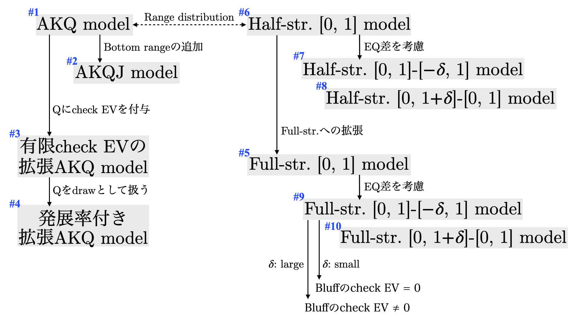
Below, we will examine these criticisms through models. Since models will appear one after another, Figure 1 provides a roadmap in advance. If you get lost, please refer to it as you read along 🧭

First, let us consider the first point of MDF criticism: the case where the caller's side has weak hands. As a concrete scenario, let us look at the following toy model called the AKQJ model.

【Model #2】 AKQJ model

- Player 1: Holds A or Q with equal probability.
- Player 2: Holds K with probability $${1-p}$$ and J with probability $${p}$$.
- Only Player 1 can bet (or check) once (= half-street), with the bet size fixed at $${B}$$ relative to the pot.
- Player 2 can call or fold against Player 1's bet; raising is not allowed.
- When Player 1 checks or Player 2 calls, a showdown occurs and the player with the higher-ranked card wins the pot at that point.

This model is almost the same as the AKQ model, but Player 2 holds not only the bluff catcher K but also J with 0% EQ. The Nash equilibrium of this model is as follows.

Nash Equilibrium of the AKQJ Model

- Player 1 always bets A, and bets Q with probability $${\frac{B}{1+B}}$$ and checks with probability $${\frac{1}{1+B}}$$.
- Player 2 calls Player 1's bet with K at probability $${\frac{1}{1+B}}$$ and folds with probability $${\frac{B}{1+B}}$$, and pure folds J.

The Nash equilibrium does not depend on the probability $${p}$$ that Player 2 holds J. This is natural because J has 0% EQ and is helpless against any of Player 1's actions. The fundamental AKQ model structure where Player 1 sandwiches K with A and Q is unaffected.

However, note that the overall call frequency of Player 2's range differs from that in the AKQ model. The overall call frequency of Player 2's range is obtained by taking a weighted average over K and J:

$$ (1-p)\cdot\frac{1}{1+B}+p\cdot 0 = (1-p)\cdot\mathrm{MDF}(B) \tag{2} $$

Thus, the overall call frequency of the range has become smaller than MDF. This is a natural result: while the caller calls K at a frequency matching MDF, J is always folded, which raises the overall fold frequency. In this way, while MDF is meaningful for a specific bluff catcher, it is suggested that the guideline "play so that the overall call frequency of your range matches MDF" is not necessarily correct. MDF criticism #1, "When there is an EQ difference between the two players' ranges (especially when the caller's side has very weak hands), MDF is not achieved," is valid.

Next, let us consider the second criticism: the case where bluff hands have nonzero EQ. As a simple model, consider the following extended AKQ model with finite check EV.

【Model #3】 Extended AKQ Model with Finite Check EV

- Player 1: Holds A or Q with equal probability.
- Player 2: Holds K.
- Only Player 1 can bet (or check) once (= half-street), with the bet size fixed at $${B}$$ relative to the pot.
- Player 2 can call or fold against Player 1's bet; raising is not allowed.
- When Player 1 checks or Player 2 calls, a showdown occurs and the player with the higher-ranked card wins the pot at that point.
- However, when Player 1 checks Q, it has $${p [100\%]}$$ EQ against Player 2's K.

In this model, the bluff hand Q is given check EV. In actual poker on the flop or turn, hands with 0% EQ essentially do not exist. For example, on the flop, even the weakest hands typically have around 10-20% EQ. What happens when we naively introduce such a situation into the model? The procedure for finding the Nash equilibrium of this model is almost the same as the standard AKQ model. To derive Player 2's K call frequency, we use the condition that Player 1's bluff hand Q has equal bet EV and check EV, but note that check EV is now $${p}$$ rather than 0. Here we show the result for when $${p}$$ is sufficiently small.

Nash Equilibrium of the Extended AKQ Model with Finite Check EV (when p is sufficiently small)

- Player 1 always bets A, and bets Q with probability $${\frac{B}{1+B}}$$ and checks with probability $${\frac{1}{1+B}}$$.
- Player 2 calls Player 1's bet with probability $${\frac{1-p}{1+B}}$$ and folds with probability $${\frac{B+p}{1+B}}$$.

Compared to the standard AKQ model, the Nash equilibrium of this model shows that Player 2's K call (fold) frequency has been modified. The call frequency is reduced by a factor of $${1-p}$$ relative to MDF. When Player 1 is dealt the bluff hand (Q), the check EV tempts them to check. In response, Player 2 reduces the bluff catching frequency to encourage Player 1 to bluff.

You might think "Well, of course the call frequency decreases below MDF if check EV is finite." But wait a moment. If the bluff hand has check EV, shouldn't we also consider the possibility of outdrawing the bluff catcher when bet and called? To address this question, let us consider the following extended AKQ model with improvement rate.

【Model #4】 Extended AKQ Model with Improvement Rate

- Player 1: Holds A or Q with equal probability.
- Player 2: Holds K.
- Only Player 1 can bet (or check) once (= half-street), with the bet size fixed at $${B}$$ relative to the pot.
- Player 2 can call or fold against Player 1's bet; raising is not allowed.
- When Player 1 checks or Player 2 calls, a showdown occurs: one community card is dealt, and the player with the stronger hand wins the pot at that point.
- The community card is Q with probability $${p}$$ and 2 with probability $${1-p}$$, and hand ranking is determined by pair > high card (within high card, ranks determine strength).

In this model, Player 1's bluff hand Q can improve with probability $${p}$$ and outdraw Player 2's bluff catcher K. As with the AKQ model, the Nash equilibrium is derived by setting the action frequencies so that K is indifferent between call and fold, and Q is indifferent between bet and check. We omit the derivation, but under the condition that the improvement rate $${p}$$ is sufficiently small, the following result is obtained.

Nash Equilibrium of the Extended AKQ Model with Improvement Rate (when p is sufficiently small)

- Player 1 always bets A, and bets Q with probability $${x}$$ and checks with probability $${1-x}$$.
- Player 2 calls Player 1's bet with probability $${y}$$ and folds with probability $${1-y}$$.

where,

$$ \begin{align*} x = \frac{1}{1-\frac{1+2B}{1+B}p}\frac{B}{1+B} \tag{3} \\ y = \frac{1-p}{1-\frac{1+2B}{1+B}p}\frac{1}{1+B} \tag{4} \end{align*} $$

Player 1's bluff frequency $${x}$$ is larger than the bluff frequency in the standard AKQ model (= $${\frac{B}{1+B}}$$). Since Player 1's bluff hand has a certain probability of being "promoted" to a value hand, more bluffing is needed to keep the opponent's K indifferent.

On the other hand, looking at Player 2's call frequency $${y}$$, it is larger than MDF (= $${\frac{1}{1+B}}$$). Player 1's bluff hand has EQ equal to $${p}$$ against the opponent's range, which creates check EV. So the bluff hand finds checking attractive, but considering that there is also a chance to outdraw after betting and being called, betting also seems attractive. In this case, betting is actually more attractive, and Player 1 is inclined to bet. In response, Player 2 increases the call frequency to discourage Player 1's bluffs.

The key point in situations where bluff hands have improvement potential is that both check and bet have their advantages. Which generates greater profit is determined by whether (average pot when betting) = (pot after being called) x (call probability) is greater than (current pot). Since (pot after being called) = $${1+2B}$$ and substituting (call probability) = MDF (= $${\frac{1}{1+B}}$$), we get (average pot when betting) = $${\frac{1+2B}{1+B} > 1}$$, which is the structure that makes betting more profitable than checking.

Looking at the results of the extended AKQ model with finite check EV and the extended AKQ model with improvement rate, they show opposite results: one decreases the call frequency below MDF and the other increases it. So which model is more realistic?

In the extended AKQ model with finite check EV, checking gives Q finite EQ, but when betting, the bluff hand's EQ is 0. In the extended AKQ model with improvement rate, the EQ is the same whether checking or betting. In reality, the truth lies between these two. For example, in a situation where you CB from IP on the flop, if you check back a very weak hand and proceed to the turn, roughly 20% EQ remains. On the other hand, if you bet that hand, the EQ drops to around 10% against the opponent's call range (depending on bet size).

Recalling the result of the extended AKQ model with finite check EV, the call frequency decreased from MDF by an amount equal to Q's post-check EQ. Assuming a flop scenario with Q's post-check EQ of 20%, the call frequency is 20% lower than MDF. On the other hand, in the extended AKQ model with improvement rate, setting the bluff hand improvement rate to 20% and considering a pot bet, equation (4) shows that the call frequency is about 14% higher than MDF. Taking the simple average of these to estimate the impact of bluff hand EQ on the flop, the call frequency against a pot bet would be about 3% lower than MDF. The effect of bluff hand EQ on the deviation of call frequency from MDF is expected to be at most a few percent. So MDF criticism #2, "Bluff hands actually have nonzero EQ (so MDF is unreliable!)," is valid but may have a surprisingly small impact.

Now let us look at how much the call frequency deviates from MDF in actual poker on the flop.

Figure 2 shows a graph of BB's defense frequency (= call frequency + raise frequency) versus bet size for CBs in SB vs. BB SRP. The red dots are plotted by calculating the defense frequency against CB averaged over all flops from GTO Wizard 50NL Complex solutions for the given spot. The black curve depicts $${\mathrm{MDF}(B)=\frac{1}{1+B}}$$ from equation (1). The data is taken from the GTO Wizard Blog article "Mathematical Misconceptions in Poker" (link).

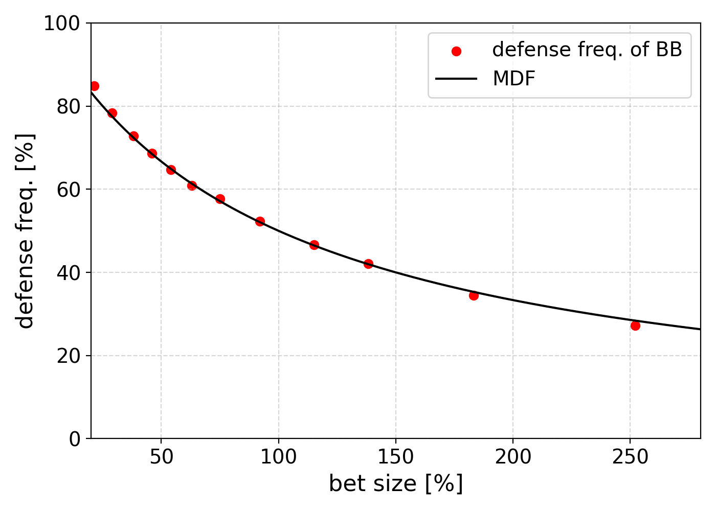
Looking at Figure 2, we can see that the call frequency averaged over all flops matches MDF beautifully. The models we have examined so far had polarized bet ranges based on the AKQ model, so we especially expect call frequencies close to MDF for large bet sizes with polarized bet ranges. Looking more carefully at Figure 2, you may notice that for large bet sizes, the call frequency is a few percent smaller than MDF.

We examined two representative factors causing call frequency to deviate from MDF: the EQ difference between the two players' ranges and the finite EQ of bluff hands. Let us estimate these effects concretely.

In SB vs. BB SRP, the EQ difference between the two ranges is about 7 points on average (SB's EQ is 53.5%, BB's EQ is 46.5%). According to equation (2) of the AKQJ model, the overall call frequency decreases by the amount of the EQ difference between the ranges. That is, this model indicates about a 7% decrease in call frequency. However, it is unnatural to assume that only the KJ side has the weakest hands and that this alone determines the overall EQ difference. In reality, EQ differences also arise from the AQ side having more A's. And even if the proportion of A's on the AQ side increases, K's call frequency on the KJ side does not change. Considering that in actual poker the overall EQ difference arises from both the bettor's top range strength and the caller's bottom range weakness, we can roughly estimate that about half of the EQ difference (~3.5%) contributes to the gap between call frequency and MDF.

What about the effect of bluff hands having finite EQ? Assuming bluff hand EQ of about 20% on the flop, we previously estimated that call frequency is about 3% lower than MDF for pot bets. As bet size increases, this deviation decreases. Based on the earlier calculations, the call frequency matches MDF exactly for double-pot bets.

Combining these factors, around double-pot bet sizes, the call frequency should be about 3% lower than MDF. Looking at the two data points with large bet sizes in Figure 2 (around 180-250%), we see roughly a 4% deviation, which shows quite good agreement with the model.

However, the remarkable point of Figure 2 is that the call frequency matches MDF not only for large bet sizes but across all bet sizes. It is puzzling why this holds so universally. Also, explaining things solely through models derived from the AKQ model feels somewhat unconvincing.

So let us consider the third point of MDF criticism: "MDF is a call frequency derived from a perfectly polarized range, as in the AKQ model." Indeed, on the flop, the EQ distributions of both ranges are similar, and it is rarely the case that the preflop aggressor's range appears polarized when looking at the EQ graph.

A well-known model that contrasts with the AKQ model from the perspective of distribution is the [0, 1] model. The [0, 1] model is one where each player's hand is randomly drawn from the closed interval $${[0, 1]}$$, and the winner is determined by the larger number. While the AKQ model had one player with an extreme range distribution of 100% and 0% EQ, the [0, 1] model gives both players uniformly distributed ranges. Below, we will use this model to discuss call frequency against bets.

In cases like SB vs. BB SRP where the OOP player is the bettor, rather than a half-street model where only one player can bet, we should consider a full-street model where both players can bet. The extended AKQ-related models we have seen were treated as half-street, but since the caller holds a condensed range, in most cases changing to full-street would not allow them to lead out, so the situation remains unchanged. However, in the [0, 1] model, the situation changes between half-street and full-street.

So, to investigate the OOP bettor case, let us start by looking at the full-street [0, 1] model.

【Model #5】 Full-street [0, 1] model

- Player 1 (OOP) and Player 2 (IP) each independently select one real number from the closed interval $${[0, 1]}$$ according to a uniform distribution.
- OOP Player 1 can first bet (or check), and if they check, IP Player 2 can also bet (or check) (= full-street). The bet size is fixed at $${B}$$ relative to the pot.
- Both players can call or fold against the opponent's bet; raising is not allowed.
- When one player's bet is called by the other, or when both check, a showdown occurs and the player with the larger initially selected number wins the pot at that point.

We omit the derivation, but the Nash equilibrium of this model is as follows.

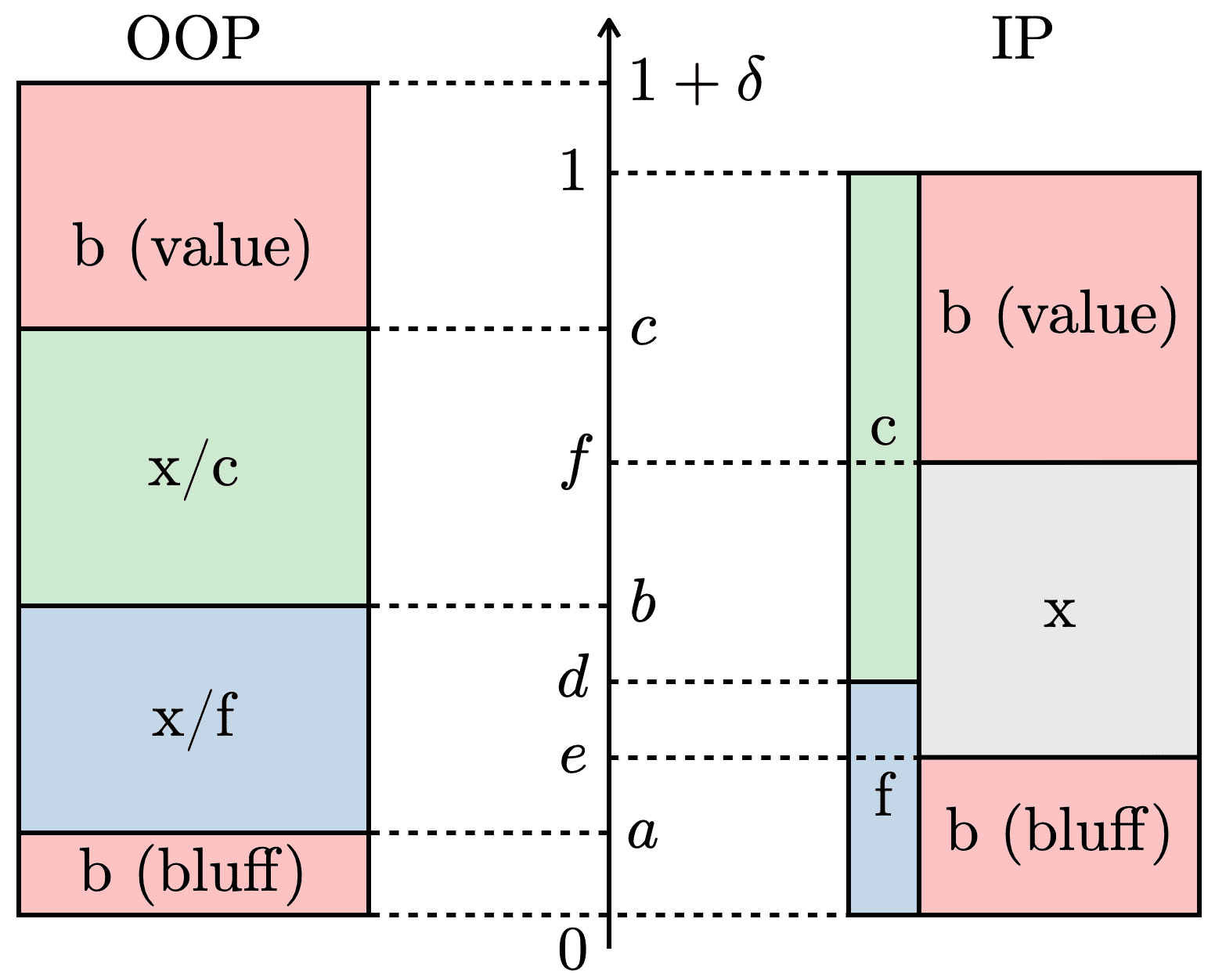
Nash Equilibrium of the Full-street [0, 1] Model

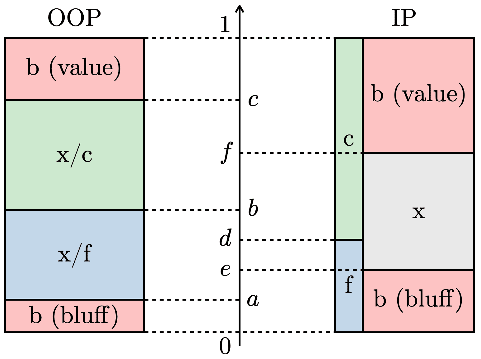
- Figure 3 shows an overview of the Nash equilibrium.
- OOP (Player 1)'s strategy has four pure strategy intervals divided by three boundaries $${a, b, c}$$. The interval $${[c, 1]}$$ is value bet, $${[b, c]}$$ is check/call, $${[a, b]}$$ is check/fold, and $${[0, a]}$$ is bluff bet.
- IP (Player 2)'s strategy when facing a bet from OOP (Player 1): call with hands in $${[d, 1]}$$, fold with hands in $${[0, d]}$$.
- IP (Player 2)'s strategy when OOP (Player 1) checks: value bet with hands in $${[f, 1]}$$, value bet with hands in $${[e, f]}$$, and bluff bet with hands in $${[0, e]}$$.

where,

$$ \begin{align*} a &= \frac{B}{(1+B)^2(1+2B)}, \tag{5} \\ b &= d = \frac{B}{1+B}, \tag{6} \\ c &= 1-\frac{1}{(1+B)(1+2B)}, \tag{7} \\ e &= \frac{B}{(1+B)(1+2B)}, \tag{8} \\ f &= 1-\frac{1}{1+2B} \tag{9} \end{align*} $$

What we want to focus on now is IP's call frequency $${1-d}$$ against OOP's bet. Referring to equation (6) from the results above, we can see that the call frequency $${1-d}$$ is exactly equal to MDF. This can actually be understood without performing the calculation. First, OOP makes polarized bets. OOP's remaining check range becomes more marginal and condensed than the original range because the top and bottom have been removed by betting. Therefore, IP's bet after OOP checks can lower the value threshold compared to OOP's bet, and accordingly, bluffs also increase. This means that IP's check-or-bluff-bet boundary hand $${e}$$ is higher than OOP's check-or-bluff-bet boundary hand $${a}$$. This implies that the EV of OOP's check-or-bluff-bet boundary hand $${a}$$ is 0. Although OOP's bluff hands might seem to have check EV, they actually do not. This means that OOP's bet and IP's call have the same structure as the standard AKQ model, and IP should call against OOP's bet at a frequency equal to MDF.

Although the full-street [0, 1] model appears complex at first glance, the call frequency itself can be derived easily from such considerations. It may be surprising that MDF appears exactly despite the full-street [0, 1] model having an entirely different range distribution from the AKQ model. It seems MDF is a more universal benchmark than expected. MDF criticism #3, "MDF is a call frequency derived from a perfectly polarized range, as in the AKQ model," may not be a 100% accurate criticism.

Being told "The AKQ model is a good model for describing the flop, and therefore IP's average call frequency against OOP's CB can be accurately obtained using MDF!!" might make you feel skeptical about using a model with such extreme range distribution. However, "The full-street [0, 1] model is a good model for describing the average flop in OOP bettor situations" seems comparatively reasonable. Alternatively, the following understanding may be helpful.

- The full-street [0, 1] model is a good model for describing the average flop in OOP bettor situations.
↓
- The structure of OOP's polarized bet and the bluff hand's check EV being 0 in the full-street [0, 1] model is the same as the AKQ model structure.
↓
- IP's call frequency equals MDF as defined from the AKQ model.

Understanding it this way, we can expect that the [0, 1] model might also describe the IP bettor case. That is, for the IP bettor case, we can predict that the half-street [0, 1] model would correspond.

From here on, we will deepen our understanding of the flop "MDF" by examining models related to the [0, 1] model. If you feel lost, please refer to the roadmap in Figure 1.

【Model #6】 Half-street [0, 1] model

- Player 1 and Player 2 each independently select one real number from the closed interval $${[0, 1]}$$ according to a uniform distribution.
- Only Player 1 can bet (or check) once (= half-street), with the bet size fixed at $${B}$$ relative to the pot.
- Both players can call or fold against the opponent's bet; raising is not allowed.
- When Player 1 checks or Player 2 calls, a showdown occurs and the player with the larger initially selected number wins the pot at that point.

The Nash equilibrium is a relatively well-known result and is as follows.

Nash Equilibrium of the Half-street [0, 1] Model

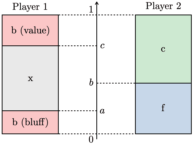
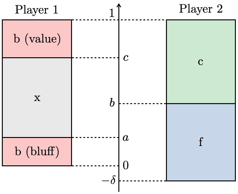
- Figure 4 shows an overview of the Nash equilibrium.
- Player 1 value bets with hands in $${[c, 1]}$$, checks with hands in $${[a, c]}$$, and bluff bets with hands in $${[0, a]}$$.
- When facing a bet from Player 1, Player 2 calls with hands in $${[b, 1]}$$ and folds with hands in $${[0, b]}$$.

where,

$$ \begin{align*} a &= \frac{B}{(1+2B)(2+B)}, \tag{10} \\ b &= 1-\frac{2(1+B)}{(1+2B)(2+B)}, \tag{11} \\ c &= 1-\frac{1+B}{(1+2B)(2+B)} \tag{12} \end{align*} $$

In the half-street [0, 1] model, just as in the full-street case, Player 1 has a polarized bet range and the corresponding caller has a strategy that switches between fold and call at a certain threshold. What we care about is the call frequency against bets $${1-b}$$, which when recalculated gives:

$$ \begin{align*} 1-b = \frac{1}{1+B}\left(1-\frac{B}{(1+2B)(2+B)}\right) \tag{13} \end{align*} $$

We notice that the call frequency in equation (13) is smaller than MDF (= $${\frac{1}{1+B}}$$) by the amount $${\frac{B}{(1+2B)(2+B)} (>0)}$$. This is due to the finite check EV of Player 1's bluff hands. To see this, let us trace the equations used to derive the Nash equilibrium of this model.

After determining the form of the Nash equilibrium as in Figure 4, we simply need each boundary hand to be indifferent between its two actions. For example, for the hand with value $${a}$$, we set up the equation so that bet EV equals check EV. That is,

$$ \begin{align*} (\text{bet EV}) &= b\cdot 1 + (1-b)\cdot (-B) \\ &= (\text{check EV}) = a \tag{14} \end{align*} $$

Rearranging this, we get:

$$ \begin{align*} 1-b = \frac{1}{1+B}(1-a) \tag{15} \end{align*} $$

Equation (15) shows that Player 2's call frequency $${1-b}$$ is reduced from MDF (= $${\frac{1}{1+B}}$$) by the amount of check EV $${a}$$. Player 1 has showdown value when checking, so they won't want to bet without a certain degree of profit. As a result, Player 2 reduces bluff catching accordingly.

This is exactly the same structure as the extended AKQ model with finite check EV. The only difference is that in this model, the check EV is not a fixed predetermined value but is determined by $${a}$$, the upper bound of bluff hands. $${a}$$ represents the total amount of bluffs, and the total amount of bluffs is determined by the total amount of value (and bet size), and the total amount of value (the lower bound of value hands) is determined by the opponent's call range. Thus, in this model, the call frequency $${1-b}$$, total bluff amount $${a}$$, and total value amount $${1-c}$$ are interrelated and ultimately determine the Nash equilibrium. Therefore, to obtain the exact call (or fold) frequency in equation (13) (or equation (11)), we solve a system of three equations including equation (15), but equation (15) is sufficient to understand how the call frequency deviates from MDF.

Now, can this half-street [0, 1] model explain the actual defense frequency (= call frequency + raise frequency) against flop CBs in real poker? Figure 5 plots the defense frequency against CB versus bet size in BTN vs. BB SRP. The red dots are plotted by calculating the defense frequency against CB averaged over all flops from GTO Wizard 50NL Complex solutions for the given spot. The black curve represents MDF from equation (1), and the blue curve represents the call frequency from equation (13) obtained from the half-street [0, 1] model.

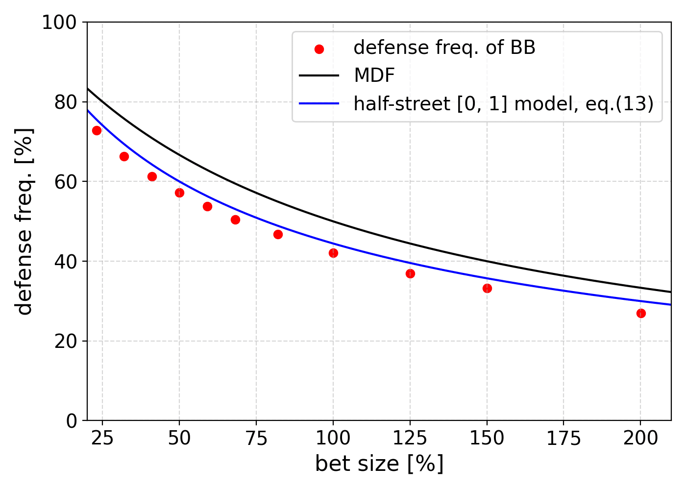
First, looking at Figure 5, we notice that when IP is the bettor, the call frequency shows a significant deviation from MDF. The call frequency is nearly 10 points below MDF across all bet sizes. This is a stark contrast to the OOP bettor case in Figure 2, where the call frequency aligned well with MDF.

How does the half-street [0, 1] model's call frequency compare? It seems to be doing fairly well. It is reasonably successful as a model for estimating call frequency in the IP bettor case. However, the half-street [0, 1] model systematically overestimates the call frequency.

Therefore, to more precisely reproduce the IP bettor situation on the flop, let us account for the EQ difference between the two players' ranges. Consider the following half-street [0, 1]-[-delta, 1] model.

【Model #7】 Half-street [0, 1]-[-delta, 1] model

- Player 1 selects from the closed interval $${[0, 1]}$$, and Player 2 selects from the closed interval $${[-\delta, 1]}$$, each independently according to a uniform distribution. Here, $${\delta}$$ is a sufficiently small positive real number.
- Only Player 1 can bet (or check) once (= half-street), with the bet size fixed at $${B}$$ relative to the pot.
- Both players can call or fold against the opponent's bet; raising is not allowed.
- When Player 1 checks or Player 2 calls, a showdown occurs and the player with the larger initially selected number wins the pot at that point.

In this model, instead of both players selecting values from the same closed interval $${[0, 1]}$$, one player has a slightly wider range extending downward to $${[-\delta, 1]}$$. In this case, Player 1's range EQ is $${\frac{1+\delta}{2}}$$ and Player 2's range EQ is $${\frac{1-\delta}{2}}$$, so the EQ difference between the two players' ranges equals $${\delta}$$.

The Nash equilibrium of this extended [0, 1] model with EQ difference is as follows.

Nash Equilibrium of the Half-street [0, 1]-[-delta, 1] Model

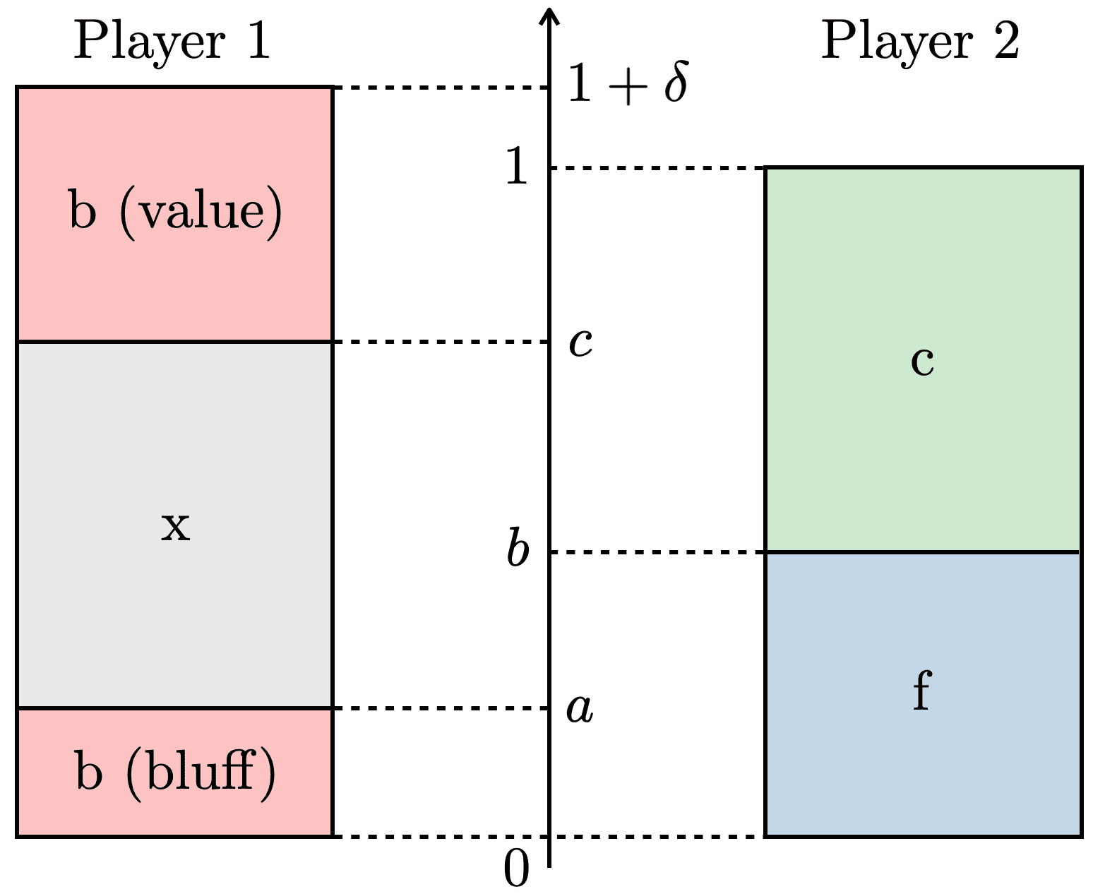
- Figure 6 shows an overview of the Nash equilibrium.
- Player 1 value bets with hands in $${[c, 1]}$$, checks with hands in $${[a, c]}$$, and bluff bets with hands in $${[0, a]}$$.
- When facing a bet from Player 1, Player 2 calls with hands in $${[b, 1]}$$ and folds with hands in $${[-\delta, b]}$$.

where,

$$ \begin{align*} a &= \frac{B}{(1+2B)(2+B)}, \tag{16} \\ b &= 1-\frac{2(1+B)}{(1+2B)(2+B)}, \tag{17} \\ c &= 1-\frac{1+B}{(1+2B)(2+B)} \tag{18} \end{align*} $$

In fact, equations (16)-(18) are equal to equations (13)-(15) of the half-street [0, 1] model and do not depend on $${\delta}$$. However, Player 2's call frequency reflects the change of range from $${[0, 1]}$$ to $${[-\delta, 1]}$$:

$$ \begin{align*} \frac{1-b}{1+\delta} = \frac{1}{1+\delta}\frac{1}{1+B}\left(1-\frac{B}{(1+2B)(2+B)}\right) \tag{19} \end{align*} $$

and depends on $${\delta}$$. Player 2 has more hands with 0% EQ, so the call frequency becomes smaller than in the half-street [0, 1] model. Within the range where $${\delta}$$ is sufficiently small, the rate of decrease in call frequency can be approximated by $${\delta}$$. For example, in the BTN vs. BB SRP case, the range EQ difference is about 6 points on average (BTN's range EQ is 53.2%, BB's range EQ is 46.8%), so $${\delta\sim 0.06}$$ and the call frequency decreases by about 6%.

Let us compare the call frequency based on equation (19) of this model with $${\delta = 0.06}$$ against the average defense frequency (= call frequency + raise frequency) in BTN vs. BB SRP. Figure 7 shows the defense frequency for the spot as red dots, the call frequency from the half-street [0, 1]-[-delta, 1] model (equation (19)) as a blue dashed line, the call frequency from the half-street [0, 1] model (equation (13)) as a blue solid line, and MDF (equation (1)) as a black solid line.

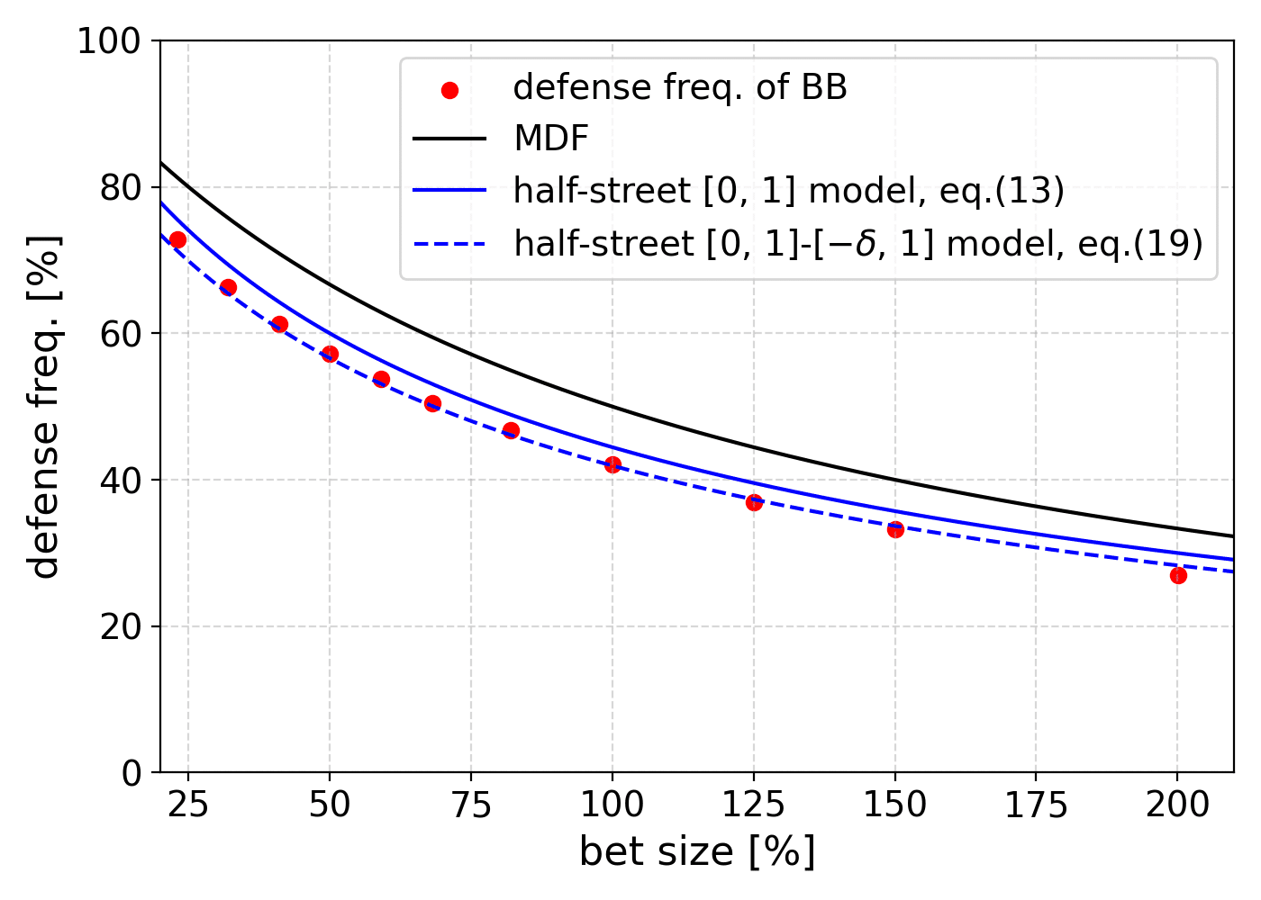
How about that? It reproduces the bet size dependence of defense frequency in BTN vs. BB SRP with quite good accuracy.

This result is very encouraging, but it is natural to wonder whether there are other ways to introduce the EQ difference between the two players' ranges. The half-street [0, 1]-[-delta, 1] model created the range EQ difference by adding 0% EQ hands to Player 2. The opposite approach would be to add 100% EQ hands to Player 1. With this in mind, consider the following half-street [0, 1+delta]-[0, 1] model.

【Model #8】 Half-street [0, 1+delta]-[0, 1] model

- Player 1 selects from the closed interval $${[0, 1+\delta]}$$, and Player 2 selects from the closed interval $${[0, 1]}$$, each independently according to a uniform distribution. Here, $${\delta}$$ is a sufficiently small positive real number.
- Only Player 1 can bet (or check) once (= half-street), with the bet size fixed at $${B}$$ relative to the pot.
- Both players can call or fold against the opponent's bet; raising is not allowed.
- When Player 1 checks or Player 2 calls, a showdown occurs and the player with the larger initially selected number wins the pot at that point.

Would this produce different results from the previous half-street [0, 1]-[-delta, 1] model? The Nash equilibrium is as follows.

Nash Equilibrium of the Half-street [0, 1+delta]-[0, 1] Model

- Figure 8 shows an overview of the Nash equilibrium.
- Player 1 value bets with hands in $${[c,1+\delta]}$$, checks with hands in $${[a, c]}$$, and bluff bets with hands in $${[0, a]}$$.
- When facing a bet from Player 1, Player 2 calls with hands in $${[b,1]}$$ and folds with hands in $${[0, b]}$$.

where,

$$ \begin{align*} a &= \frac{B}{(1+2B)(2+B)}(1+2(1+B)\delta), \tag{20} \\ b &= 1-\frac{2(1+B(1-\delta))}{(1+2B)(2+B)}, \tag{21} \\ c &= 1-\frac{1+B(1-\delta)}{(1+2B)(2+B)} \tag{22} \end{align*} $$

Player 2's call frequency is:

$$ \begin{align*} 1-b = \frac{1}{1+B}\left(1-\frac{B}{(1+2B)(2+B)}(1+2(1+B)\delta)\right) \tag{23} \end{align*} $$

which can be confirmed to be smaller than the call frequency from the half-street [0, 1] model (equation (13)). We can see that when the bettor has a range EQ advantage over the caller, the call frequency generally tends to decrease. When the bettor's top range is strengthened, more value hands can be constructed, which in turn increases the amount of bluff hands used, raising the upper bound (= EQ) of bluff hands. Then, bluff hands have higher check EV and would prefer to check when possible. In response, the caller lowers the call frequency to encourage more bluffing.

The notion that the call frequency decreases because the bettor's top range is strengthened is not entirely obvious. In fact, in the AKQ model, even if the ratio of A to Q is changed from 1:1 to, say, 1.2:1, K's call frequency does not change from MDF. In the current half-street [0, 1+delta]-[0, 1] model, the key is that increasing value quantity raises both the bluff quantity and check EV, which pushes the opponent's call frequency downward. In the AKQ model, no matter how much value hand quantity increases, the bluff hand's check EV remains at 0, so the opponent's call frequency is always fixed regardless of the top range details.

For the half-street [0, 1] model, we introduced the range EQ difference between the two players in two ways: adding bottom range to the caller and adding top range to the bettor. Let us plot and compare the differences between these two methods of introducing EQ difference.

Figure 9 shows the defense frequency against CB in BTN vs. BB SRP as red dots, the call frequency from the half-street [0, 1+delta]-[0, 1] model (equation (23)) as a blue dash-dot line, the call frequency from the half-street [0, 1]-[-delta, 1] model (equation (19)) as a blue dashed line, the call frequency from the half-street [0, 1] model (equation (13)) as a blue solid line, and MDF (equation (1)) as a black solid line. All models use $${\delta=0.06}$$.

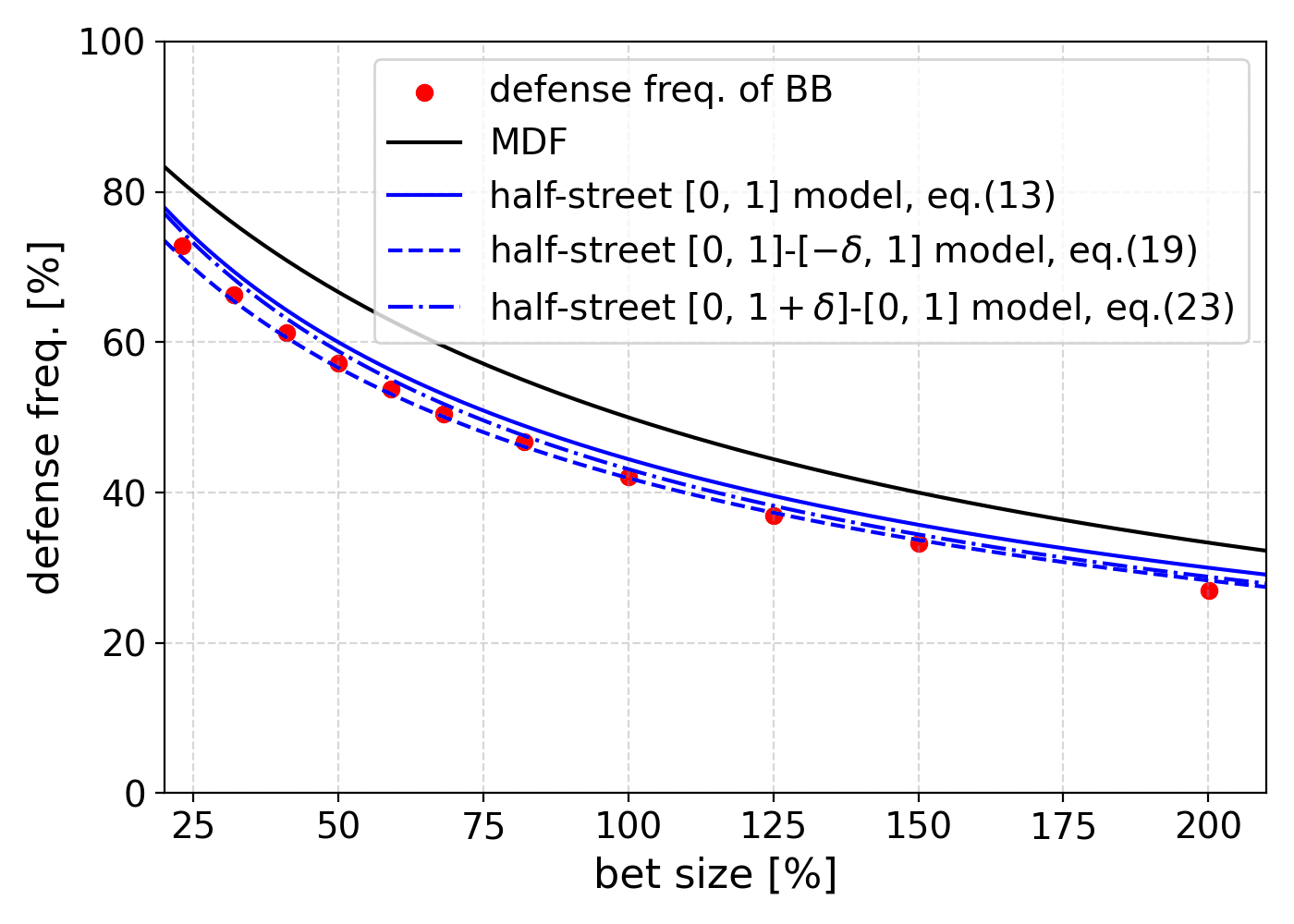
We omit the detailed derivation, but when $${B\delta < 1}$$, the call frequency is evaluated lower in equation (19) (adding bottom range to the caller) than in equation (23) (adding top range to the bettor). This aligns with intuition, as adding 0% EQ hands to the caller more directly impacts call frequency.

In actual poker, EQ differences arise from both the bettor's top range and the caller's bottom range, so reality lies between equations (19) and (23). Looking at Figure 9, equation (19) (blue dashed line) fits the red data points better than equation (23) (blue dash-dot line). In other words, for defense frequency against CB in BTN vs. BB SRP, equation (19) provides the more accurate estimate.

In any case, it is fair to say that the average defense frequency against flop CBs in the IP bettor case is well described by the EQ-corrected half-street [0, 1] model.

We would like to say "happily ever after," but some of you may have the following question: "In the OOP bettor case, the full-street [0, 1] model suggested that defense frequency is well approximated by MDF, but wouldn't introducing EQ differences there also cause the theoretical value to deviate from MDF?"

This is a perfectly reasonable question, so let us verify it.

First, let us consider adding 0% EQ hands to IP's bottom range. We will work with the following full-street [0, 1]-[-delta, 1] model.

【Model #9】 Full-street [0, 1]-[-delta, 1] model

- OOP (Player 1) selects from the closed interval $${[0, 1]}$$, and IP (Player 2) selects from the closed interval $${[-\delta, 1]}$$, each independently according to a uniform distribution. Here, $${\delta}$$ is a sufficiently small positive real number.
- OOP Player 1 can first bet (or check), and if they check, IP Player 2 can also bet (or check) (= full-street). The bet size is fixed at $${B}$$ relative to the pot.
- Both players can call or fold against the opponent's bet; raising is not allowed.
- When one player's bet is called by the other, or when both check, a showdown occurs and the player with the larger initially selected number wins the pot at that point.

Although it looks somewhat complex, the Nash equilibrium of this model can be derived by hand.

Nash Equilibrium #1 of the Full-street [0, 1]-[-delta, 1] Model (when delta is sufficiently small)

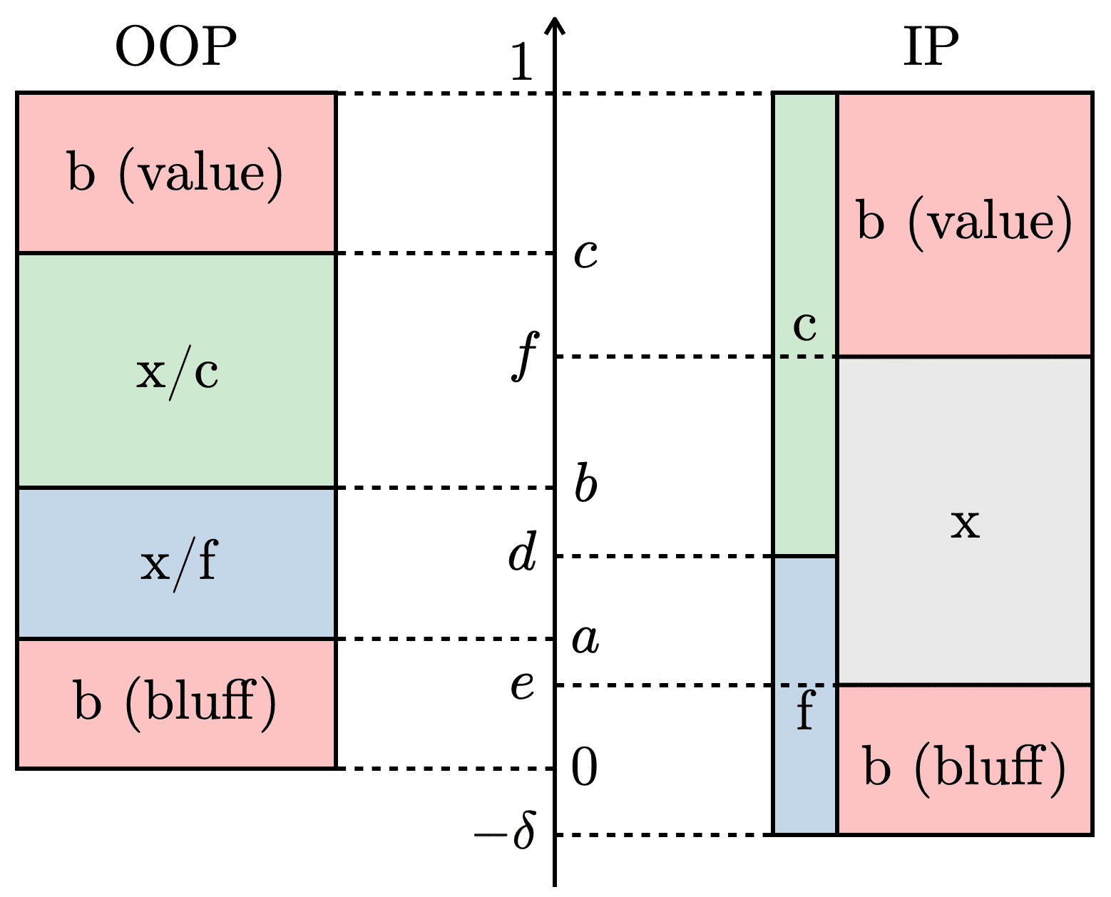
- Figure 10 shows an overview of the Nash equilibrium.
- OOP (Player 1)'s strategy has four pure strategy intervals divided by three boundaries $${a, b, c}$$. The interval $${[c, 1]}$$ is value bet, $${[b, c]}$$ is check/call, $${[a, b]}$$ is check/fold, and $${[0, a]}$$ is bluff bet.
- IP (Player 2)'s strategy when facing a bet from OOP (Player 1): call with hands in $${[d, 1]}$$, fold with hands in $${[0, -\delta]}$$.
- IP (Player 2)'s strategy when OOP (Player 1) checks: value bet with hands in $${[f, 1]}$$, value bet with hands in $${[e, f]}$$, and bluff bet with hands in $${[-\delta, e]}$$.

where,

$$ \begin{align*} a &= \frac{B}{(1+B)^2(1+2B)}(1+\delta), \tag{24} \\ b &= d = \frac{B-\delta}{1+B}, \tag{25} \\ c &= 1-\frac{1+\delta}{(1+B)(1+2B)}, \tag{26} \\ e &= -\delta + \frac{B}{(1+B)(1+2B)}(1+\delta), \tag{27} \\ f &= 1-\frac{1+\delta}{1+2B} \tag{28} \end{align*} $$

IP's call frequency against OOP's bet is:

$$ \begin{align*} \frac{1-d}{1+\delta} = \frac{1}{1+B} \tag{29} \end{align*} $$

which equals MDF. In the standard full-street [0, 1] model as well, the call frequency in equation (6) matched MDF. The key common point is that OOP's boundary hand between bluff and check/fold is weaker than IP's check-back range after OOP checks.

Sharp readers may have already noticed: could adding bottom range to IP create finite check EV for OOP's bluff hands? In other words, when $${\delta}$$ is sufficiently small, $${a<e}$$ holds and OOP's bluff hands have no check EV, but if $${\delta}$$ is increased, could $${a>e}$$ reverse and give OOP's bluff hands check EV (causing IP's call frequency to deviate from MDF)?

This observation is indeed correct. The Nash equilibrium shown above was derived under the assumption that $${\delta}$$ is sufficiently small, fixing the range partition as in Figure 10. Let us investigate when this Nash equilibrium breaks down.

From equations (24) and (27),

$$ \begin{align*} e-a = \frac{1}{(1+B)^2(1+2B)}(B^2-\delta (1+4B+4B^2+2B^3)) \tag{30} \end{align*} $$

so the Nash equilibrium of Figure 10 holds when:

$$ \begin{align*} \delta \leq \frac{B^2}{1+4B+4B^2+2B^3} \tag{31} \end{align*} $$

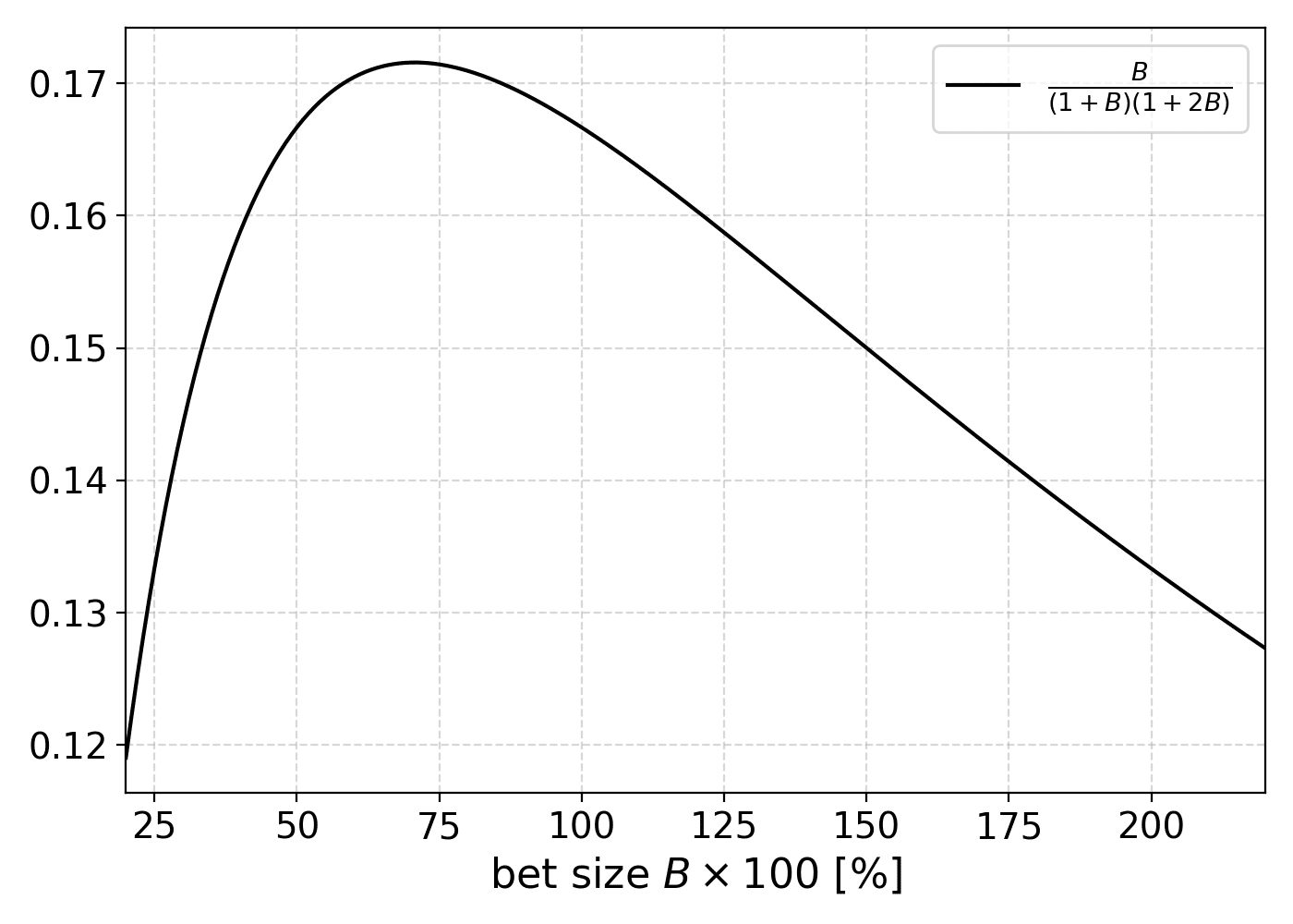
Plotting the right-hand side of equation (31) as a function of $${B}$$ gives Figure 11.

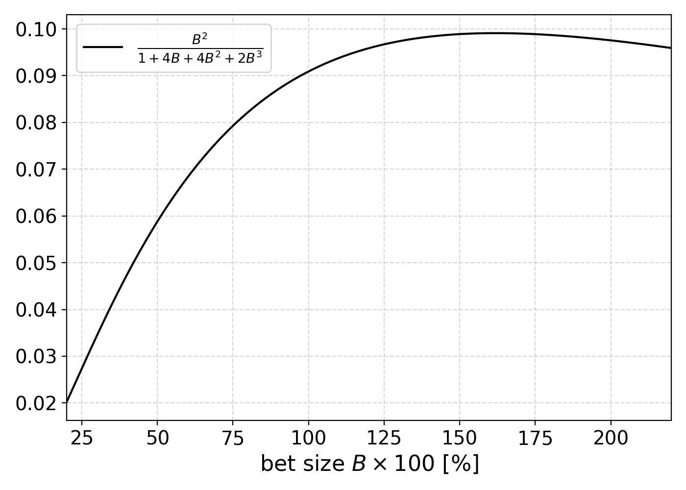
With SB vs. BB SRP in mind, the EQ difference gives $${\delta\sim 0.05}$$, so for bet sizes of approximately 45% or more, condition (31) is satisfied and the Nash equilibrium shown above holds.

Let us also look at the Nash equilibrium when condition (31) is violated.

Nash Equilibrium #2 of the Full-street [0, 1]-[-delta, 1] Model (when delta is slightly larger)

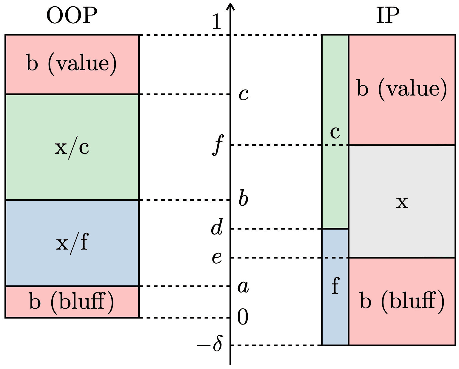
- Figure 12 shows an overview of the Nash equilibrium.
- OOP (Player 1)'s strategy has four pure strategy intervals divided by three boundaries $${a, b, c}$$. The interval $${[c, 1]}$$ is value bet, $${[b, c]}$$ is check/call, $${[a, b]}$$ is check/fold, and $${[0, a]}$$ is bluff bet.
- IP (Player 2)'s strategy when facing a bet from OOP (Player 1): call with hands in $${[d, 1]}$$, fold with hands in $${[-\delta, d]}$$.
- IP (Player 2)'s strategy when OOP (Player 1) checks: value bet with hands in $${[f, 1]}$$, value bet with hands in $${[e, f]}$$, and bluff bet with hands in $${[-\delta, e]}$$.

where,

$$ \begin{align*} a &= \frac{B}{1+4B+4B^2+2B^3}, \tag{32} \\ b &= d = \frac{B}{1+B}\left( 1-\frac{B}{1+4B+4B^2+2B^3} \right), \tag{33} \\ c &= 1-\frac{1+B}{1+4B+4B^2+2B^3}, \tag{34} \\ e &= -\delta + \frac{B(1+B)}{1+4B+4B^2+2B^3}, \tag{35} \\ f &= 1-\frac{(1+B)^2}{1+4B+4B^2+2B^3} \tag{36} \end{align*} $$

Comparing Figure 12 with Figure 10, you can see that the relative positions of $${a}$$ and $${e}$$ are reversed in Nash equilibrium #2. The qualification "when delta is slightly larger" is because further increasing $${\delta}$$ beyond the violation of (31) will eventually reverse the relationship between $${\delta}$$ and $${a}$$, collapsing the check/fold range, but this is not central to the main discussion and can be ignored.

In this Nash equilibrium, IP's call frequency is:

$${b}$$

Under the condition $$ \begin{align*} \frac{1-d}{1+\delta} = \frac{1}{1+B}\left( 1 - \frac{1}{1+\delta}\left( \delta - \frac{B^2}{1+4B+4B^2+2B^3} \right) \right) \tag{37} \end{align*} $$ for this Nash equilibrium to hold, the parenthetical expression in the second term of equation (37) is non-negative, so IP's call frequency is smaller than MDF. This is the familiar structure where finite check EV for OOP's bluff hands causes IP's call frequency to decrease.

As with the half-street case, let us also examine a model that introduces EQ difference by adding top range to OOP.

【Model #10】 Full-street [0, 1+delta]-[0, 1] model

- Player 1 selects from the closed interval $${a\geq e}$$, and Player 2 selects from the closed interval $${[0, 1+\delta]}$$, each independently according to a uniform distribution. Here, $${[0, 1]}$$ is a sufficiently small positive real number.
- OOP Player 1 can first bet (or check), and if they check, IP Player 2 can also bet (or check) (= full-street). The bet size is fixed at $${\delta}$$ relative to the pot.
- Both players can call or fold against the opponent's bet; raising is not allowed.
- When one player's bet is called by the other, or when both check, a showdown occurs and the player with the larger initially selected number wins the pot at that point.

Let us examine the Nash equilibrium when $${B}$$ is sufficiently small. The derivation under this assumption follows exactly the same approach as the full-street [0, 1] model.

Nash Equilibrium of the Full-street [0, 1+delta]-[0, 1] Model (when delta is sufficiently small)

- Figure 13 shows an overview of the Nash equilibrium.
- OOP (Player 1)'s strategy has four pure strategy intervals divided by three boundaries $${\delta}$$. The interval $${a, b, c}$$ is value bet, $${[c, 1+\delta]}$$ is check/call, $${[b, c]}$$ is check/fold, and $${[a, b]}$$ is bluff bet.
- IP (Player 2)'s strategy when facing a bet from OOP (Player 1): call with hands in $${[0, a]}$$, fold with hands in $${[d, 1]}$$.
- IP (Player 2)'s strategy when OOP (Player 1) checks: value bet with hands in $${[0, d]}$$, value bet with hands in $${[f, 1]}$$, and bluff bet with hands in $${[e, f]}$$.

where,

$${[0, e]}$$

From the Nash equilibrium of Figure 13's form, OOP's bluff hands have no check EV, and IP's call frequency equals MDF (equation (39)).

When deriving the Nash equilibrium, we assumed $$ \begin{align*} a &= \frac{B}{1+B}\left( \frac{1}{(1+B)(1+2B)} + \delta \right), \tag{38} \\ b &= d = \frac{B}{1+B}, \tag{39} \\ c &= 1-\frac{1}{(1+B)(1+2B)}, \tag{40} \\ e &= \frac{B}{(1+B)(1+2B)}, \tag{41} \\ f &= 1-\frac{1}{1+2B} \tag{42} \end{align*} $$ was sufficiently small to fix the form of Figure 13, but as with the full-street [0, 1]-[-delta, 1] model, the relative positions of $${\delta}$$ and $${a}$$ could potentially reverse. Let us check when this occurs.

Taking the difference between $${e}$$ and $${e}$$, from equations (38) and (41),

$${a}$$

so the Nash equilibrium of Figure 13 holds if and only if:

$$ \begin{align*} e-a = \frac{B}{1+B}\left( \frac{B}{(1+B)(1+2B)} - \delta \right) \tag{43} \end{align*} $$

Plotting the right-hand side of equation (44) as a function of $$ \begin{align*} \delta \leq \frac{B}{(1+B)(1+2B)} \tag{44} \end{align*} $$ gives Figure 14.

With $${B}$$ in mind, condition (44) is well satisfied for bet sizes of at least approximately 20% to 200%. "Even when OOP's top range is strengthened and value hands increase, the effect of lowering IP's call frequency is small" — a result similar to that of the half-street [0, 1+delta]-[0, 1] model.

What the full-street [0, 1]-[-delta, 1] model and full-street [0, 1+delta]-[0, 1] model tell us is that in the OOP bettor case, the change in call frequency due to range EQ difference is smaller than in the IP bettor case. In the OOP bettor case, even adding IP's bottom range has limited impact on IP's call frequency, and adding OOP's top range produces no change in IP's call frequency for reasonable bet sizes.

Based on the above observations, we can propose that as a unified model for explaining the average call frequency against flop CBs, the [0, 1] model extended to account for EQ differences should be used.

In the OOP bettor case, the full-street [0, 1] model with EQ differences applies, and IP's call frequency (essentially) matches MDF (equation (1)).

$${\delta\sim 0.05}$$

[Note: "(Essentially)" is because, as seen in the full-street [0, 1]-[-delta, 1] model, a Nash equilibrium where the bluff hand's check EV remains finite due to adding IP's bottom range may hold. We previously discussed that for $$ \begin{align*} \mathrm{MDF}(B) = \frac{1}{1+B}. \tag{1} \end{align*} $$, IP's call frequency matches MDF for bet sizes of approximately 45% or more. This estimate assumes all range EQ difference is attributed to IP's bottom range, but in reality, EQ differences also come from the amount of OOP's top range. Taking this into account, this Nash equilibrium is realized for a very broad range of bet sizes.]

In the IP bettor case, the half-street [0, 1] model with EQ differences applies, and adopting the half-street [0, 1]-[-delta, 1] model as a specific method of introducing EQ difference, OOP's call frequency follows equation (19).

$${\delta\sim 0.05}$$

In particular, let us call equation (19) the corrected MDF as a new concept.

Let us once again present the relationships among the models discussed in this article [Figure 1].

Finally, let us look at some concrete examples to wrap up.

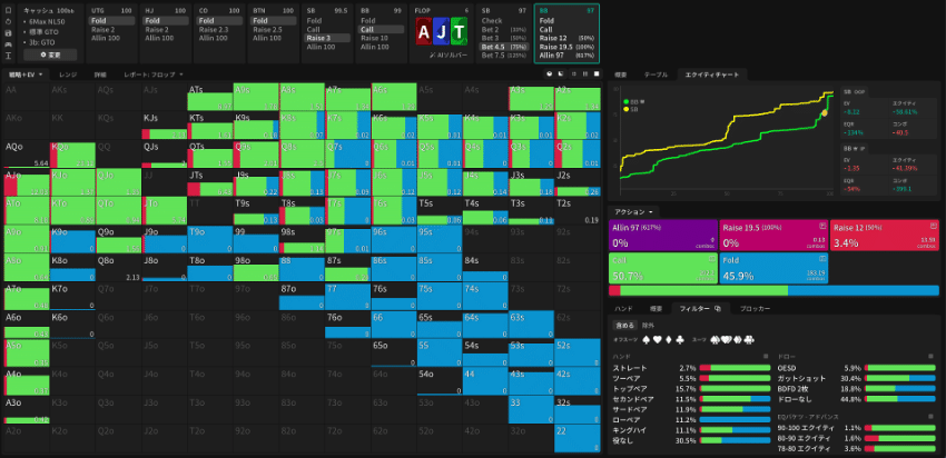
Since we primarily discussed how call frequency changes when EQ differences are considered, let us look at an example where this is prominent. Figure 15 shows flops sorted by BTN's range EQ from highest to lowest in BTN vs. BB SRP (solutions are from GTO Wizard cash 100bb, 6max NL50, GTO-GTO). The AJTr flop produces BTN range EQ of 57.9%, which appears to create the largest EQ difference. Let us examine this one.

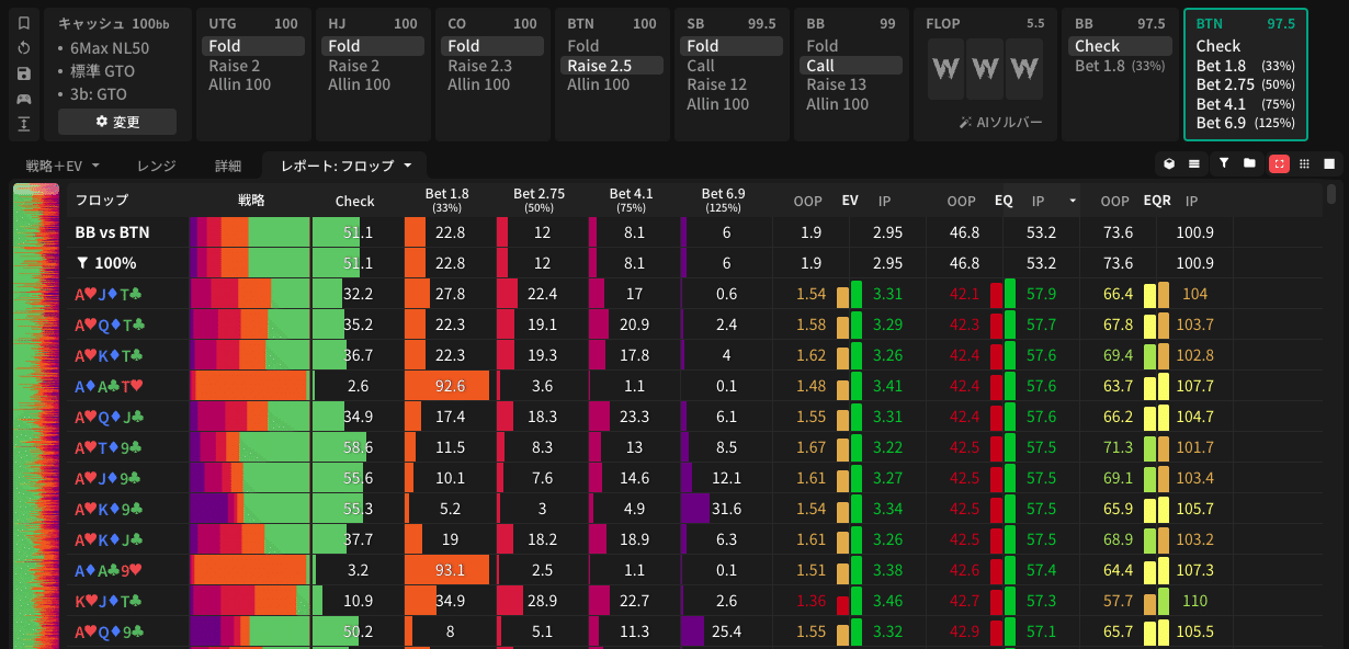
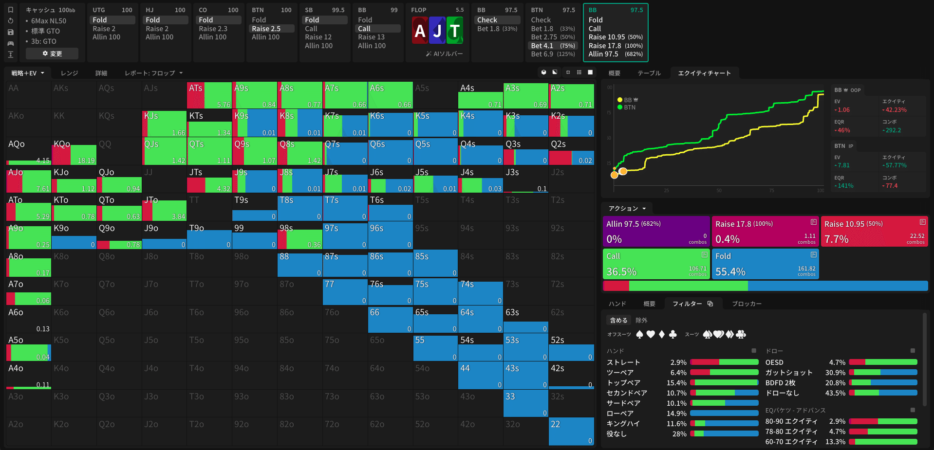
Figure 16 shows BB's strategy after BTN bets a 75% pot CB on AJTr in BTN vs. BB SRP. BB's defense frequency is 44.6% and fold frequency is 55.4%.

According to MDF, $$ \begin{align*} \frac{1-b}{1+\delta} = \frac{1}{1+\delta}\frac{1}{1+B}\left(1-\frac{B}{(1+2B)(2+B)}\right). \tag{19} \end{align*} $$, giving a defense frequency of 57.1% and fold frequency of 42.9%. This overestimates the defense frequency by 12.5 points. In reality, players fold much more than MDF suggests. This is the kind of spot where people often complain "MDF is not achieved!"

In this article, we argued that the extended [0, 1] model with EQ differences is a good model for estimating flop defense frequency. For the IP bettor case, the conclusion was that the corrected MDF (equation (19)) from the half-street [0, 1]-[-delta, 1] model is optimal for evaluating OOP's defense frequency. Substituting bet size $${\frac{1}{1+3/4}=4/7\simeq 0.571}$$ and the EQ difference $${B=3/4}$$ for this flop into equation (19), we obtain a defense frequency of 44.0% and fold frequency of 56.0%. This estimates the actual defense (or fold) frequency with remarkable accuracy.

Let us look at the same flop with positions changed to SB vs. BB SRP. Figure 17 shows BB's strategy after SB bets a 75% pot CB on AJTr in SB vs. BB SRP. BB's defense frequency is 54.1% and fold frequency is 45.9%. We can see that more hands are defended compared to the BTN vs. BB case. In the OOP bettor case, we should consider the full-street [0, 1+delta]-[0, 1] model or the full-street [0, 1]-[-delta, 1] model, and the former yields MDF as OOP's defense frequency. Indeed, MDF of 57.1% is relatively close to the actual defense frequency of 54.1%, with only about a 3-point difference. For the latter model, we discussed two different Nash equilibria [Figure 1], but since the EQ difference is large in this case, we use equation (37) and substitute $${B=3/4}$$ and $${\delta = 0.135}$$ to obtain a defense frequency of 54.3% and fold frequency of 45.7%. This is very close to the actual defense (fold) frequency, demonstrating that the EQ-extended full-street [0, 1] model is successful as a model for estimating defense frequency against OOP's CB.

3. Summary

In this article, we examined the Nash equilibria of 10 models as shown in Figure 1, investigating how call (or fold) frequency changes under various conditions. In particular, we argued that the [0, 1] model extended to account for EQ differences is a good model for estimating the average defense frequency against flop CBs. As average behavior across all flops, we found that in the OOP bettor (IP caller) case, the call frequency matches MDF (equation (1)), while in the IP bettor (OOP caller) case, the call frequency is lower than MDF and can be described by the corrected MDF (equation (19)). We also concretely demonstrated the applicability not only to average behavior but also to individual flops.

Let us conclude with some caveats.

First, while we argued that the EQ-extended [0, 1] model is an effective toy model for describing defense frequency against CBs, note that it is not a universal model that can explain every property of poker flops. For example, it cannot describe flop CB frequency, CB size, or hand selection for CB. In the extended [0, 1] model, the bet range is always polarized, but in reality, hands with moderate EQ also bet, and nuts don't always bet. Does this mean the model is wrong? Not necessarily. One perspective (prediction) is that while actual flop bet ranges are wider than what the model suggests, the majority of defense frequency against bets is determined by the composition of high-EQ and low-EQ hands in the bet range (which gives the model a degree of validity).

Additionally, there are several points not considered (or not fully addressed) in the models presented here. Bet range polarization (= degree of polarization) is one. Others include the existence of raises and subsequent streets such as the turn and river, which may affect fold frequency against bets. Interested readers may find it worthwhile to explore these topics.

Regarding the estimation of defense frequency for individual flops, it should also be noted that the EQ-extended [0, 1] model is not infallible. Naturally, there are cases where the defense frequency suggested by the model diverges from the actual frequency. Considering this, we used the expression "applicability" in the summary section. In the models presented here, defense frequency can be calculated using only bet size and range EQ difference as inputs [note: strictly speaking, there was some arbitrariness in model selection regarding how to introduce the EQ difference], and if this were effective for most individual flops, that would be remarkable. It is a fact that it succeeds for at least a certain number of individual flops, and we believe there is a reasonable consensus that range EQ difference, in addition to bet size, is important when considering defense frequency against CBs.

In the Weekly Equilibrium (@GTOmaga) published in 2025 by Amu and Drama, which gained significant attention, the approach to estimating fold (or defense) frequency against flop CBs is described as follows:

Step 1. Determine fold frequency from bet size. (Considering EQ difference)
Step 2. Assess your range and select hands to fold starting from the weakest.
Step 3. Determine whether the hand you hold should be folded.

(Quoted from "Weekly Equilibrium" Stage 1-3 Call Decision Equilibrium Thinking EQ Difference)

As shown, the approach is to estimate fold frequency based on bet size and range EQ difference, which is consistent with the proposal in this article. Furthermore,

Judging specifically how many percent to shift, or which hands to fold, is largely a matter that requires experience.

(Quoted from "Weekly Equilibrium" Stage 1-3 Call Decision Equilibrium Thinking EQ Difference)

Regarding this point, we hope that the fold (or defense) frequency estimates from the models presented in this article will serve as one quantitative guideline.

4. Related Literature

Here are some references related to MDF.

• glass's note article "Why You Can Fold More Than 50% Against Pot Bet" (link)
  -> This article provides detailed derivations for the half-street [0, 1] model discussed here, explaining why MDF is not achieved against pot bets and why folding more than 50% is acceptable.

• Wagon_man's note article "Why MDF and GTO Diverge" (link)
  -> This article points out the check EV perspective on why solver defense frequencies deviate from MDF, and introduces specific spots.

• Wagon_man's note article "Strictly Following MDF Against Raises" (link)
  -> This article briefly explains the principle that MDF should be nearly always followed against raises.

• GTO Wizard Blog "Mathematical Misconceptions in Poker" (link)
  -> This compares how fold frequency changes with bet size for IP bettor and OOP bettor cases, including definitions of MDF and alpha. Data from this article was also used in this article.

• GTO Wizard YouTube channel "The Most Misunderstood Poker Metric" (link)
  -> This broadly explains the divergence between solver defense frequency and MDF, the relationship between defense frequency against raises and MDF, and their qualitative reasoning. The content largely overlaps with the Wizard Blog above but with more detailed explanations and demonstrations.

5. Conclusion

This article has been very long, but thank you for reading this far. We suspect many readers may have skipped ahead to this section. Even if the details were unclear, we would be happy if you take away that "defense frequency against CBs can be roughly estimated by considering bet size and EQ difference," and that this kind of model-based analysis exists for understanding poker. Model calculations help expand what we consider "obvious" in poker.

The inspiration for the MDF-related content in this article came from the Q&A forum in the Seeker Start Discord server. We would like to express our gratitude to those who asked sharp questions about MDF and to those who contributed to the discussions. If you are interested in joining the Discord server, please send a DM to Seeker Start (@seekerstart).