Nash Equilibrium in Multiway Pots and Equilibrium Selection Theory

Author: Sigma (Twitter: @sigm_4)

What You'll Learn

• What properties Nash equilibria generally have in multiway pots, and why strategies contained in multiway Nash equilibria cannot be called GTO strategies

• Extending the AKQ game to multiway

• The concept of MDF sharing

• Which strategies to adopt from multiple Nash equilibria, and which strategies are selected in GTO Wizard

Introduction: Nash Equilibrium in Multiway

Recently, GTO Wizard began offering 3-way solutions, which has attracted considerable attention.

https://blog.gtowizard.com/gto_wizard_ai_3_way_benchmarks/

In this article, we explain fundamental aspects of equilibrium strategies in multiway pots (particularly 3-way). Specifically, we discuss MDF sharing—one of the basic concepts—through model-based analysis to understand foundational multiway strategy. We also concretely verify that strategies contained in multiway Nash equilibria generally do not possess the desirable properties needed to be called GTO strategies (optimal strategies). In particular, when multiple Nash equilibria exist, we discuss which Nash equilibrium should be selected and how the solver (GTO Wizard) makes this selection.

Extending the AKQ Game to Multiway

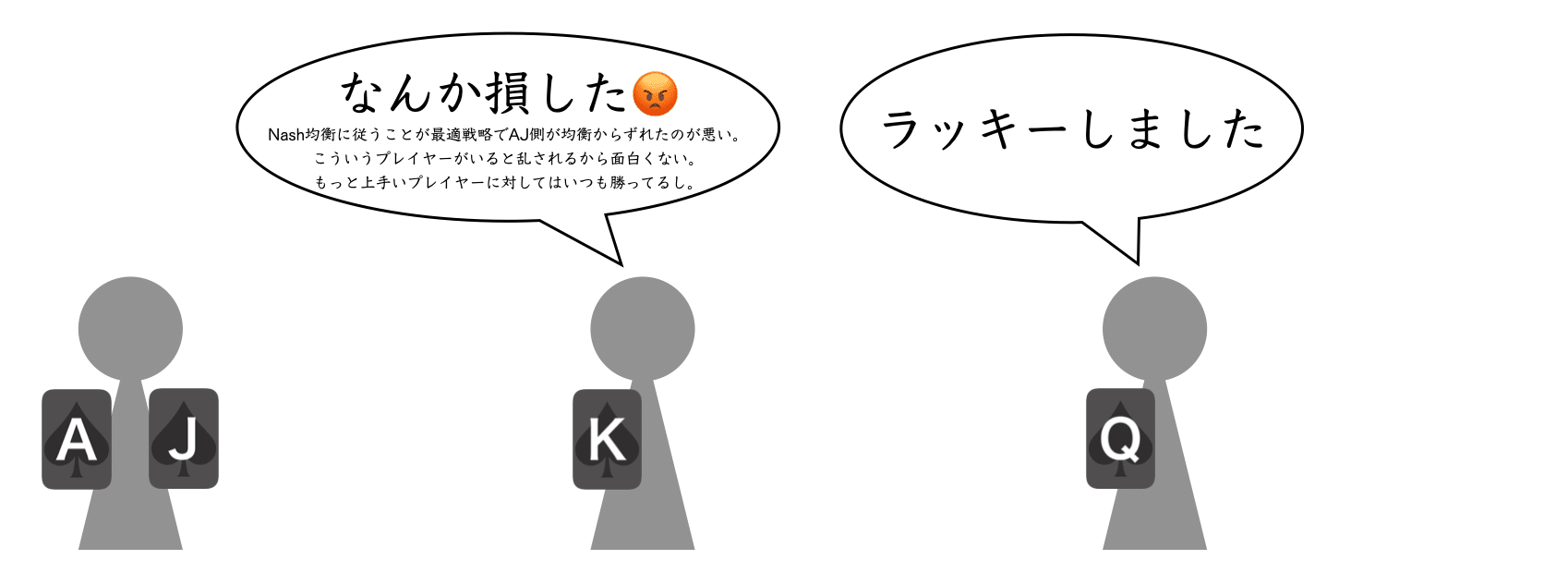
First, we consider extending the AKQ game—one of the most fundamental models in heads-up poker—to multiway. Below, we examine the most basic 3-way scenario with two different variants: ① the AJ-Q-K game and ② the AJ-K-Q game.

① AJ-Q-K Game

Consider the following 3-way model setup.

・Consider a 1-street model with three players: Player 1, 2, and 3.
・Set the pot size to 1 and all players' stacks to $${S}$$.
・Players act in the order: Player 1 (BB) → Player 2 (UTG) → Player 3 (BTN).
・Each player can only check or go all in on their turn, and can call or fold against an all in.

・Player 1 (BB) holds A or J with equal probability.
・Player 2 (UTG) holds Q.
・Player 3 (BTN) holds K.

The Nash equilibrium of this AJ-Q-K game is as follows.

・Player 1 (BB with A or J) pure bets A and bets J at a frequency of $${\alpha_S:=\frac{S}{1+S}}$$.
・Player 2 (UTG with Q) pure folds against Player 1's bet, and pure checks against Player 1's check.
・Player 3 (BTN with K) calls at frequency $${1-\alpha_S}$$ and folds at frequency $${\alpha_S}$$ against Player 1's bet (after Player 2's fold). Against Player 1's check (and Player 2's check), any action is acceptable.

This is illustrated in Figure 1.

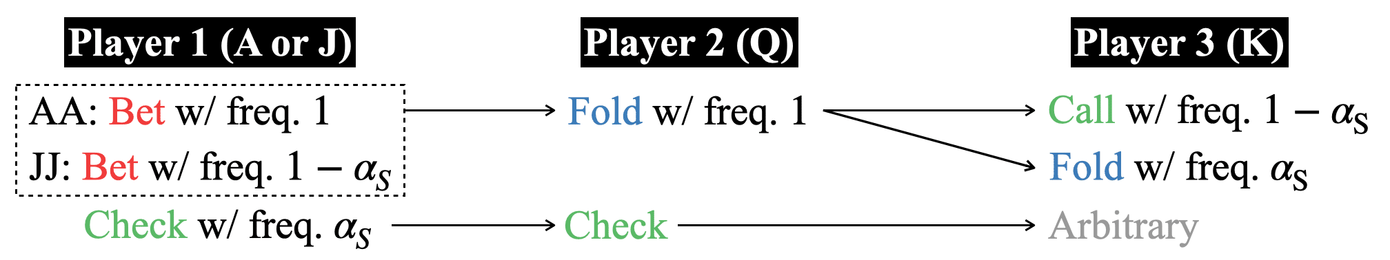
In this model, Player 1 has a polarized range against Players 2 and 3. At Nash equilibrium, as in the 2-player AKQ game, Player 1 bets value and bluffs in a ratio of $${1:\alpha_S}$$. Player 2, holding the weaker catching hand, is forced into a pure fold due to the disadvantageous middle position in the action order. After Player 2's fold, Player 3 calls at MDF $${1-\alpha_S}$$ for bet size $${S}$$, just as in the 2-player AKQ game.

When facing Player 1's bet, Player 2 might feel indifferent between calling and folding. However, since Player 3 (acting later) holds a stronger catching hand, Player 3 profits by overcalling on top of Player 2's call, which in turn causes Player 2 to lose. From Player 2's perspective, the value/bluff ratio relative to the bet size is skewed toward value, making Q's call unprofitable in terms of odds.

② AJ-K-Q Game

What happens if we swap the hands of Players 2 and 3 from the AJ-Q-K game? That is, consider the following AJ-K-Q game.

・Consider a 1-street model with three players: Player 1, 2, and 3.
・Set the pot size to 1 and all players' stacks to $${S}$$.
・Players act in the order: Player 1 (BB) > Player 2 (UTG) > Player 3 (BTN).
・Each player can only check or go all in on their turn, and can call or fold against an all in.

・Player 1 (BB) holds A or J with equal probability.
・Player 2 (UTG) holds K.
・Player 3 (BTN) holds Q.

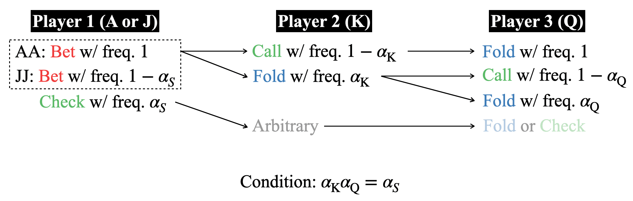
The Nash equilibrium of this AJ-K-Q game is as follows. The case after Player 1's check is trivial and omitted.

・Player 1 (BB with A or J) pure bets A and bets J at a frequency of $${\alpha_S=\frac{S}{1+S}}$$.
・For Player 2 (UTG with K), let the call frequency against Player 1's bet be $${1-\alpha_{\mathrm{K}}}$$ and the fold frequency be $${\alpha_{\mathrm{K}}}$$.
・For Player 3 (BTN with Q), let the call frequency when Player 2 folds after Player 1's bet be $${1-\alpha_{\mathrm{Q}}}$$ and the fold frequency be $${\alpha_{\mathrm{Q}}}$$. When Player 2 calls Player 1's bet, Player 3 pure folds.
・Any pair of $${\alpha_{\mathrm{K}}}$$ and $${\alpha_{\mathrm{Q}}}$$ satisfying $${\alpha_{\mathrm{K}}\alpha_{\mathrm{Q}}=\alpha_S}$$ constitutes a Nash equilibrium.

This is illustrated in Figure 2.

We can see that the Nash equilibrium differs from the AJ-Q-K game in ①. The condition for forming a Nash equilibrium,

$$ \alpha_{\mathrm{K}}\alpha_{\mathrm{Q}}=\alpha_S\quad\quad (1) $$

can be understood as follows. The probability that both Players 2 and 3 fold against Player 1's bet is $${\alpha_{\mathrm{K}}\alpha_{\mathrm{Q}}}$$, in which case Player 1 wins the pot of 1. On the other hand, the probability that Player 2 or 3 calls is $${1-\alpha_{\mathrm{K}}\alpha_{\mathrm{Q}}}$$, and if Player 1 holds the bluff hand J, they lose the bet amount of $${S}$$. For Player 1's J to be indifferent between betting and checking, $${\alpha_{\mathrm{K}}}$$ and $${\alpha_{\mathrm{Q}}}$$ must be set so that equation (1) holds.

In the 2-player AKQ game, K folded at frequency $${\alpha_S}$$ (= alpha) corresponding to bet size $${S}$$ and called at frequency $${1-\alpha_S}$$ (= MDF) to make the bluff hand (Q) indifferent between betting and checking. In the 3-player AJ-K-Q game, since there are two callers, they only need to cooperate to achieve MDF together. This is the concept called "MDF sharing."

An important note: since all pairs of $${\alpha_{\mathrm{K}}}$$ and $${\alpha_{\mathrm{Q}}}$$ satisfying equation (1) constitute Nash equilibria, there are continuously infinitely many Nash equilibria. While multiple Nash equilibria can exist in 2-player zero-sum games as well, in multiway the existence of multiple Nash equilibria creates serious problems, as we will see in the following sections.

Problems with Nash Equilibrium in Multiway

The Nash equilibria obtained from the AJ-K-Q game in ② actually do not possess the desirable properties needed to be called GTO strategies (or optimal strategies). Specifically, two issues arise.

• Even if a player follows a Nash equilibrium strategy, the EV obtained from that strategy is not guaranteed as a minimum. That is, even when one player adopts a Nash equilibrium strategy, other players can change their strategies to reduce that player's EV.

• If each player adopts a strategy from a different Nash equilibrium within the set of multiple Nash equilibria, the resulting strategy profile is not necessarily a Nash equilibrium. In other words, mixing and matching strategies from different Nash equilibria may not be permissible.

The first point about minimum EV guarantee can be easily demonstrated using model ②. First, in any Nash equilibrium, the EVs of Players 1, 2, and 3 are respectively:

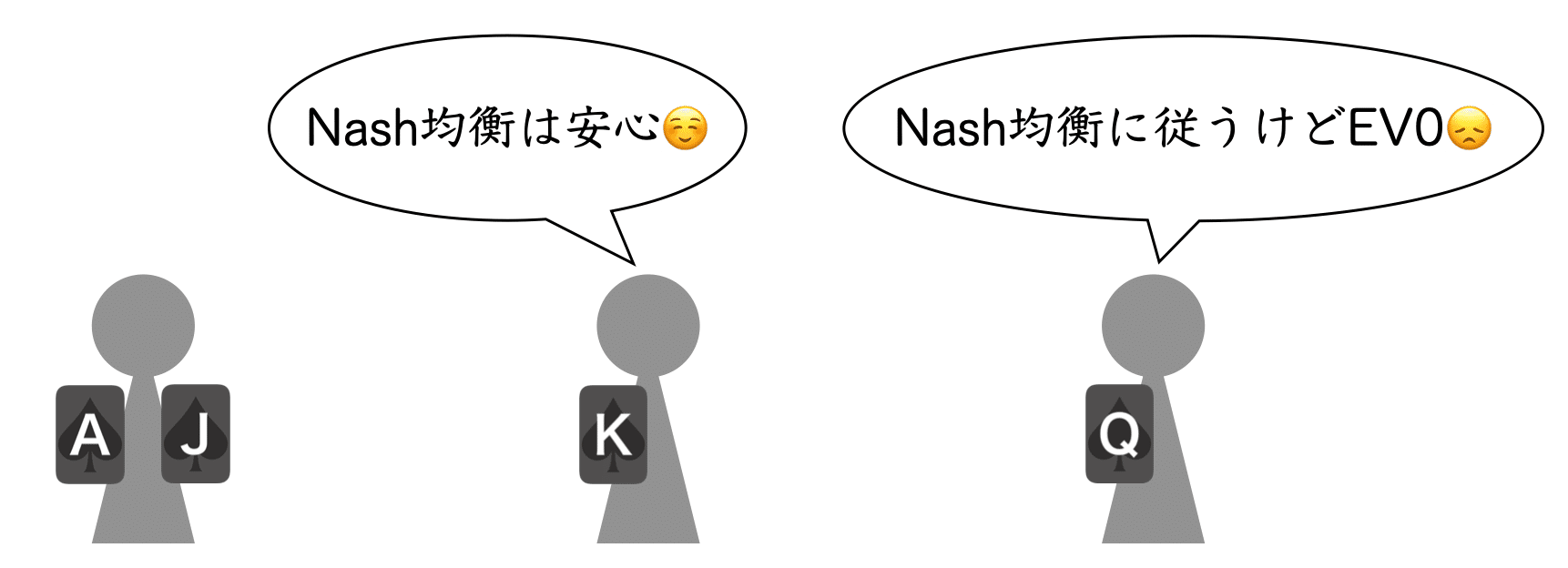
$$ \begin{align*} \mathrm{EV}_{\mathrm{AJ}}^{\mathrm{NE}} &= \frac{1+\alpha_S}{2} \\ \mathrm{EV}_{\mathrm{K}}^{\mathrm{NE}} &= \frac{1-\alpha_S}{2} \quad\quad (2) \\ \mathrm{EV}_{\mathrm{Q}}^{\mathrm{NE}} &= 0 \end{align*} $$

(The superscript NE is added to explicitly indicate Nash equilibrium.) Now consider the case where Player 1 changes strategy to pure bet both A and J. If Players 2 and 3 continue to follow the original Nash equilibrium, each player's EV changes as follows.

$$ \begin{align*} \mathrm{EV}_{\mathrm{AJ}}' &= \frac{1+\alpha_S}{2} \\ \mathrm{EV}_{\mathrm{K}}' &= \frac{1-\alpha_{\mathrm{K}}}{2} \quad\quad (3) \\ \mathrm{EV}_{\mathrm{Q}}' &= \frac{\alpha_{\mathrm{K}} -\alpha_S}{2} \end{align*} $$

Player 1's EV has not changed due to the strategy change, but Player 2's EV has decreased, while Player 3's EV has increased in return. Despite Player 2 believing they were playing a safe Nash equilibrium strategy, Player 1 unilaterally reduced Player 2's EV [Figure 3]. Intuitively, this happens because Player 2 had a lower call frequency than the MDF in the 2-player AKQ game, so when Player 1 increased their bluff frequency, Player 2's EV dropped. However, the EV difference flows not to Player 1 but to Player 3. Player 3 originally had zero EV, but because Player 1 began betting with a bluff-heavy ratio relative to the appropriate value/bluff ratio, Player 3 can now profit from calling.
[Note 1: It is often explained that two or more players can collude to reduce another player's EV, but in reality, EV transfer can occur from a single player's strategy change alone.]
[Note 2: The strategy profile after Player 1's change is of course not a Nash equilibrium. That is, Player 2 (or 3) can further change their strategy to increase their own EV.]

The second point regarding mixing strategies from different Nash equilibria can also be easily demonstrated using the AJ-K-Q game from ②. For example, the fold frequencies $${(\alpha_{\mathrm{K}}, \alpha_{\mathrm{Q}}) = (1, \alpha_S)}$$ and $${(\alpha_{\mathrm{K}}, \alpha_{\mathrm{Q}}) = (\alpha_S, 1)}$$ each satisfy equation (1) and thus constitute two different Nash equilibria. Mixing these to create the strategy profiles $${(\alpha_{\mathrm{K}}, \alpha_{\mathrm{Q}}) = (1, 1)}$$ and $${(\alpha_{\mathrm{K}}, \alpha_{\mathrm{Q}}) = (\alpha_S, \alpha_S)}$$—neither satisfies equation (1), so they are naturally not Nash equilibria. More specifically, in the case $${(\alpha_{\mathrm{K}}, \alpha_{\mathrm{Q}}) = (1, 1)}$$ (i.e., Players 2 and 3 pure fold against Player 1's bet), Player 1 can increase EV by pure betting their entire range. Conversely, in the case $${(\alpha_{\mathrm{K}}, \alpha_{\mathrm{Q}}) = (\alpha_S, \alpha_S)}$$ (i.e., Players 2 and 3 each call according to MDF against Player 1's bet), Player 1 can increase EV by reducing their bluff frequency to zero.

The first problem—that EV when adopting a Nash equilibrium strategy does not guarantee a minimum achievable EV—and the second problem—that mixing strategies from different Nash equilibria does not necessarily form a Nash equilibrium—neither occurs in 2-player zero-sum games. In 2-player zero-sum games, Nash equilibria (all strategies contained within them) always possess the desirable properties to be called GTO strategies (optimal strategies). (Indeed, it is natural to define GTO strategy in 2-player zero-sum games as any strategy contained in a Nash equilibrium.) These topics are well summarized in an article by maspy. The Wizard blog also provides discussion on the properties of multiway Nash equilibria with explanations through a 3-player Kuhn poker model.

Given these facts, in practice, beyond simply reproducing Nash equilibria, perspectives such as "whether other players understand multiway-specific Nash equilibrium (strategic guidelines)," "what kind of strategies other players are (presumably) employing," and "how plays cause EV to flow from one player to another" become even more critical in multiway.

Equilibrium Selection and Local Stability

In the previous section, we noted that multiple Nash equilibria generally exist and that in multiway games, mixing strategies from different Nash equilibria may not be permissible. So, among those multiple Nash equilibria, does a superior one exist?

In fact, such refinement and selection of Nash equilibria has been vigorously discussed. For example, Selten (1975)'s trembling-hand perfect equilibrium selected robust Nash equilibria as strategies that remain best responses even against opponents' infinitesimal mistakes (perturbations). Kreps & Wilson (1982)'s perfect Bayesian equilibrium achieved temporal consistency through sequential rationality and Bayes-rule-based belief consistency in dynamic games (extensive-form games), thereby eliminating unrealistic "threats" at zero-probability information sets (often called nodes in poker) that are permitted in Nash equilibria. Additionally, Carlsson & van Damme (1993) presented a framework for selecting risk-dominant, safer Nash equilibria from among multiple equilibria by adding noise following an appropriate distribution to each player's payoffs and taking the limit as the variance approaches zero.

There are many criteria and methodologies for selecting superior Nash equilibria from the multiple that exist. In this article, we propose local stability against strategic perturbations as a criterion for Nash equilibrium selection. Through this, we argue that from the continuous set of Nash equilibria in the AJ-K-Q game, the symmetric solution (where Players 2 and 3 have equal fold frequencies against Player 1's bet) is selected.

Recall that in the Nash equilibrium of the AJ-K-Q game, the fold frequencies of Players 2 and 3 against Player 1's bet satisfy equation (1): $${\alpha_{\mathrm{K}}\alpha_{\mathrm{Q}}=\alpha_S}$$. Take any pair $${(\alpha_{\mathrm{K}}^*,\alpha_{\mathrm{Q}}^*)}$$ satisfying this condition. We introduce small i.i.d. perturbations to this pair. That is,

$$ \begin{cases} \alpha_{\mathrm{K}}^* &\to \alpha_{\mathrm{K}}^* + \delta_{\mathrm{K}} \\ \alpha_{\mathrm{Q}}^* &\to \alpha_{\mathrm{Q}}^* + \delta_{\mathrm{Q}} \end{cases} \quad\quad (4) $$

We add $${\delta_{\mathrm{X}}\;(\mathrm{X}=\mathrm{K, Q})}$$ to the fold frequencies, where the expectation and variance are respectively

$$ E[\delta_{\mathrm{X}}] = 0, V[\delta_{\mathrm{X}}] = \sigma_{\mathrm{X}}^2 \quad\quad (5) $$

following some distribution (with $${\sigma_{\mathrm{X}} \ll 1}$$). This perturbation causes Players 2 and 3 to deviate from Nash equilibrium. We select the pair $${(\alpha_{\mathrm{K}}^*,\alpha_{\mathrm{Q}}^*)}$$ that minimizes the joint EV loss (i.e., the total EV loss of Players 2 and 3).

First, Player 1's EV at Nash equilibrium, referring again to equation (2), is

$$ \mathrm{EV}_{\mathrm{AJ}}^{\mathrm{NE}} = \frac{1+\alpha_S}{2} \quad\quad (2)' $$

If Players 2 and 3 deviate from Nash equilibrium to fold frequencies that do not satisfy equation (1), in the case $${\alpha_{\mathrm{K}}\alpha_{\mathrm{Q}} > \alpha_S}$$ (overfolding), Player 1's MES (= maximally exploitative strategy) is to pure bet the bluff hand J. Conversely, in the case $${\alpha_{\mathrm{K}}\alpha_{\mathrm{Q}} < \alpha_S}$$ (overcalling), Player 1's MES is to reduce the bluff frequency to zero. Then, Player 1's EV under MES is:

$$ \mathrm{EV}_{\mathrm{AJ}}^{\mathrm{MES}} =  \begin{cases} \frac{1+\alpha_{\mathrm{K}}\alpha_{\mathrm{Q}}}{2} & (\alpha_{\mathrm{K}}\alpha_{\mathrm{Q}} > \alpha_S) \\ \frac{1+S(1-\alpha_{\mathrm{K}}\alpha_{\mathrm{Q}})}{2} & (\alpha_{\mathrm{K}}\alpha_{\mathrm{Q}} < \alpha_S) \end{cases} \quad\quad (6) $$

Then, Player 1's additional EV under MES, from equations (2)' and (5), is:

$$ \Delta EV_{\mathrm{AJ}} := \mathrm{EV}_{\mathrm{AJ}}^{\mathrm{MES}} - \mathrm{EV}_{\mathrm{AJ}}^{\mathrm{NE}} =  \begin{cases} \frac{1}{2}(\alpha_{\mathrm{K}}\alpha_{\mathrm{Q}} - \alpha_S) & (\alpha_{\mathrm{K}}\alpha_{\mathrm{Q}} > \alpha_S) \\ \frac{S}{2}(\alpha_S - \alpha_{\mathrm{K}}\alpha_{\mathrm{Q}}) & (\alpha_{\mathrm{K}}\alpha_{\mathrm{Q}} < \alpha_S) \\ \end{cases} \quad\quad (7) $$

Since the AJ-K-Q game is zero-sum, the joint EV loss of Players 2 and 3 equals equation (7), and we need to minimize equation (7) under perturbations of the fold frequencies. When perturbations exist,

$$ \alpha_{\mathrm{K}}^*\alpha_{\mathrm{Q}}^* \to \alpha_{\mathrm{K}}^*\alpha_{\mathrm{Q}}^* + \alpha_{\mathrm{K}}^*\delta_{\mathrm{Q}} + \alpha_{\mathrm{Q}}^*\delta_{\mathrm{K}} + \delta_{\mathrm{K}}\delta_{\mathrm{Q}} \quad\quad (8) $$

and neglecting the fourth term $${\delta_{\mathrm{K}}\delta_{\mathrm{Q}}}$$ under the small perturbation assumption ($${\sigma_{\mathrm{X}}\ll 1}$$), the expected joint EV loss is:

$$ \begin{align*} E[\Delta \mathrm{EV}_{\mathrm{AJ}}] &= \frac{1}{2}\left(\alpha_{\mathrm{K}}^*\left. E[\delta_{\mathrm{Q}}]\right |_{\delta_{\mathrm{Q}}>0} + \alpha_{\mathrm{Q}}^*\left. E[\delta_{\mathrm{K}}]\right |_{\delta_{\mathrm{K}}>0}\right) - \frac{S}{2}\left(\alpha_{\mathrm{K}}^*\left. E[\delta_{\mathrm{Q}}]\right |_{\delta_{\mathrm{Q}}<0} + \alpha_{\mathrm{Q}}^*\left. E[\delta_{\mathrm{K}}]\right |_{\delta_{\mathrm{K}}<0}\right) \\ &= \frac{1+S}{4}\left(\alpha_{\mathrm{K}}^* E|\delta_{\mathrm{Q}}| + \alpha_{\mathrm{Q}}^* E|\delta_{\mathrm{K}}|\right) + \frac{1-S}{4}\left(\alpha_{\mathrm{K}}^* E[\delta_{\mathrm{Q}}] + \alpha_{\mathrm{Q}}^* E[\delta_{\mathrm{K}}]\right) \end{align*} \quad\quad (9) $$

where we used

$$ \begin{align*} E[\delta_{\mathrm{X}}] &= \left.E[\delta_{\mathrm{X}}]\right |_{\delta_{\mathrm{X}}>0} + \left.E[\delta_{\mathrm{X}}]\right |_{\delta_{\mathrm{X}}<0} \\ E|\delta_{\mathrm{X}}| &= \left.E[\delta_{\mathrm{X}}]\right |_{\delta_{\mathrm{X}}>0} - \left.E[\delta_{\mathrm{X}}]\right |_{\delta_{\mathrm{X}}<0} \end{align*} \quad\quad (10) $$

Since $${E[\delta_{\mathrm{X}}]=0}$$ (equation (5)) and we assume the same distribution for $${\delta_{\mathrm{K}}}$$ and $${\delta_{\mathrm{Q}}}$$, equation (9) simplifies to:

$$ E[\Delta \mathrm{EV}_{\mathrm{AJ}}] = \frac{1+S}{4}(\alpha_{\mathrm{K}}^* + \alpha_{\mathrm{Q}}^*) E|\delta_{\mathrm{X}}|　\quad\quad (11) $$

By the AM-GM inequality,

$$ \alpha_{\mathrm{K}}^* + \alpha_{\mathrm{Q}}^* \geq 2\sqrt{\alpha_{\mathrm{K}}^*\alpha_{\mathrm{Q}}^*} = 2\sqrt{\alpha_S} \quad\quad (12) $$

and the fold frequencies that achieve the minimum are:

$$ \alpha_{\mathrm{K}}^* = \alpha_{\mathrm{Q}}^* = \sqrt{\alpha_S} \quad\quad (13) $$

When infinitesimal perturbations are introduced equally to both players, the unique Nash equilibrium where both players have equal fold frequencies is endorsed. In this analysis, we evaluated the superiority of Nash equilibria through local stability via perturbations around the equilibrium, but as introduced earlier, there are various criteria for selecting Nash equilibria, and different equilibria may be selected depending on the situation and assumptions. In fact, for example, if we assume different distributions for the perturbations to Players 2 and 3, Nash equilibria with different fold frequencies are endorsed (roughly, the relative magnitudes of fold frequencies are determined by the relative magnitudes of the distributions' variances).

Equilibrium Solutions from the Solver (GTO Wizard) and Their Properties

So, when multiple equilibria exist, which one does the solver (GTO Wizard) select? Given inputs (ranges, bet sizes, etc.), the solver basically outputs a single equilibrium each time (within the margin of error). Particularly for the 3-way solutions introduced in GTO Wizard, since mixing strategies from different equilibria is not permissible, knowing what properties the selected equilibrium has is extremely important. In this section, we discuss what tendencies the equilibria output from GTO Wizard exhibit, based on the quantal response equilibrium (QRE) used in GTO Wizard. For details on QRE, see the following article↓↓

In this section, we use the logit QRE (LQRE)—one model of QRE—for our explanation (see the article above for details on Logit QRE).

In LQRE, the selection probability of each action is determined exponentially based on that action's EV (given the opponent's strategy is fixed). Each player's rationality is controlled by a non-negative parameter called the rationality parameter; the limit as this parameter approaches 0 gives a completely irrational equilibrium, while the limit as it approaches $${\infty}$$ gives a completely rational equilibrium. By taking a sufficiently large rationality parameter, LQRE approaches some subset of Nash equilibria. While GTO Wizard has not disclosed that LQRE is adopted as the QRE model, it obtains QRE close to Nash equilibrium through this kind of mechanism.

Below, we derive the LQRE for the AJ-K-Q game. Let $${p_{\mathrm{A}}}$$ be the bet frequency of Player 1's A, $${\alpha_{\mathrm{J}}}$$ be the bet frequency of J, $${\alpha_{\mathrm{K}}}$$ be Player 2's fold frequency against Player 1's bet, $${\alpha_{\mathrm{Q}}}$$ be Player 3's fold frequency when Player 2 folds, and $${\alpha_{\mathrm{Q}}'}$$ be Player 3's fold frequency when Player 2 calls.

After Player 1's bet, the EVs of Player 2 calling or folding are respectively:

$$ \begin{align*} \mathrm{EV}_{\mathrm{K;bc}} &= \frac{1}{p_{\mathrm{A}}+\alpha_{\mathrm{J}}}\cdot(-S) + \frac{\alpha_{\mathrm{J}}}{p_{\mathrm{A}}+\alpha_{\mathrm{J}}}\cdot(1+S+(1-\alpha_{\mathrm{Q}}')\cdot S) \\ \mathrm{EV}_{\mathrm{K;bf}} &= 0 \end{align*} \quad\quad (14) $$

After Player 1's bet and Player 2's fold, the EVs of Player 3 calling or folding are respectively:

$$ \begin{align*} \mathrm{EV}_{\mathrm{Q;bfc}} &= \frac{1}{p_{\mathrm{A}}+\alpha_{\mathrm{J}}}\cdot(-S) + \frac{\alpha_{\mathrm{J}}}{p_{\mathrm{A}}+\alpha_{\mathrm{J}}}\cdot(1+S) \\ \mathrm{EV}_{\mathrm{Q;bff}} &= 0 \end{align*} \quad\quad (15) $$

The difference between equations (14) and (15) arises from the case where Player 3 also calls after Player 2's call, which appears in the last term of $${\mathrm{EV}_{\mathrm{K;bc}}}$$ in equation (14).

After Player 1's bet and Player 2's call, the EVs of Player 3 calling or folding are respectively:

$$ \begin{align*} \mathrm{EV}_{\mathrm{Q;bcc}} &= -S \\ \mathrm{EV}_{\mathrm{Q;bcf}} &= 0 \end{align*} \quad\quad (16) $$

Therefore, considering the LQRE self-consistency equation for bet-call-fold, with rationality parameter $${\lambda}$$:

$$ \alpha_{\mathrm{Q}}' = \frac{e^{\lambda\cdot\mathrm{EV}_{\mathrm{Q;bcf}}}}{e^{\lambda\cdot\mathrm{EV}_{\mathrm{Q;bcc}}} + e^{\lambda\cdot\mathrm{EV}_{\mathrm{Q;bcf}}}} = \left(1+e^{-S\lambda}\right)^{-1} \quad\quad (17) $$

To consider equilibrium solutions close to Nash equilibrium, we take sufficiently large $${\lambda}$$. Then equation (17) becomes:

$$ \alpha_{\mathrm{Q}}' \sim 1-e^{-S\lambda} \quad\quad (18) $$

and the bet-call-fold frequency approaches its limit value of 1 exponentially. This type of exponential asymptotic behavior is observed in cases that would be pure strategies at Nash equilibrium (→reference). Applying this to equation (14):

$$ \begin{align*} \mathrm{EV}_{\mathrm{K;bc}} &= \frac{1}{p_{\mathrm{A}}+\alpha_{\mathrm{J}}}\cdot(-S) + \frac{\alpha_{\mathrm{J}}}{p_{\mathrm{A}}+\alpha_{\mathrm{J}}}\cdot(1+S+Se^{-S\lambda}) \end{align*} \quad\quad (19) $$

The final term originating from bet-call-call decays exponentially to 0 due to equation (18). Therefore, in the limit of infinite rationality parameter, the EV expressions for Players 2 and 3 (equations (14)-(15)) rapidly converge. This indicates that the LQRE self-consistency equations for Players 2 and 3's fold frequencies $${\alpha_{\mathrm{K}}, \alpha_{\mathrm{Q}}}$$ coincide, yielding $${\alpha_{\mathrm{K}}= \alpha_{\mathrm{Q}}}$$. Although the AJ-K-Q game originally has continuously infinitely many Nash equilibria, the Nash equilibrium as the limit of LQRE is the unique symmetric solution satisfying $${\alpha_{\mathrm{K}}= \alpha_{\mathrm{Q}}}$$.
[Note: More generally, the Nash equilibrium as the limit of QRE is not necessarily unique. The solution may have multiple branches, and limit values can exist separately for each branch.]

Why was this symmetric solution selected? Naively, one could say it is because Players 2 and 3 become approximately symmetric in the $${\lambda\to\infty}$$ limit. Here, we take an alternative perspective through the lens of mixed strategy entropy. As discussed in the "Supplement: Statistical Mechanics Analogy" section of the QRE article, the problem of finding LQRE can be reformulated as a free energy minimization problem by viewing the rationality parameter as inverse temperature. Free energy consists of internal energy and entropy; internal energy represents the (negated) EV of the (mixed) strategy in poker, while entropy represents the randomness (information content) of the mixed strategy. Since all continuously existing infinitely many Nash equilibria yield the same internal energy (EV), in the $${\lambda\to\infty}$$ limit each player tries to select a strategy that increases entropy to lower free energy. In general, the entropy of player $${i}$$'s mixed strategy $${P_i}$$ is written as:

$$ S(P_i) = -\sum_{a_i}P_i(a_i)\ln P_i(a_i) \quad\quad (20) $$

Equation (20) achieves its maximum when the frequency $${P_i(a_i)}$$ is set equally across all actions $${a_i}$$, so in the AJ-K-Q game, Players 2 and 3 each aim to bring their fold frequency closer to 1/2. However, due to the constraint of equation (1), both players cannot achieve this simultaneously, and as a result, they compromise by balancing their fold frequencies equally.

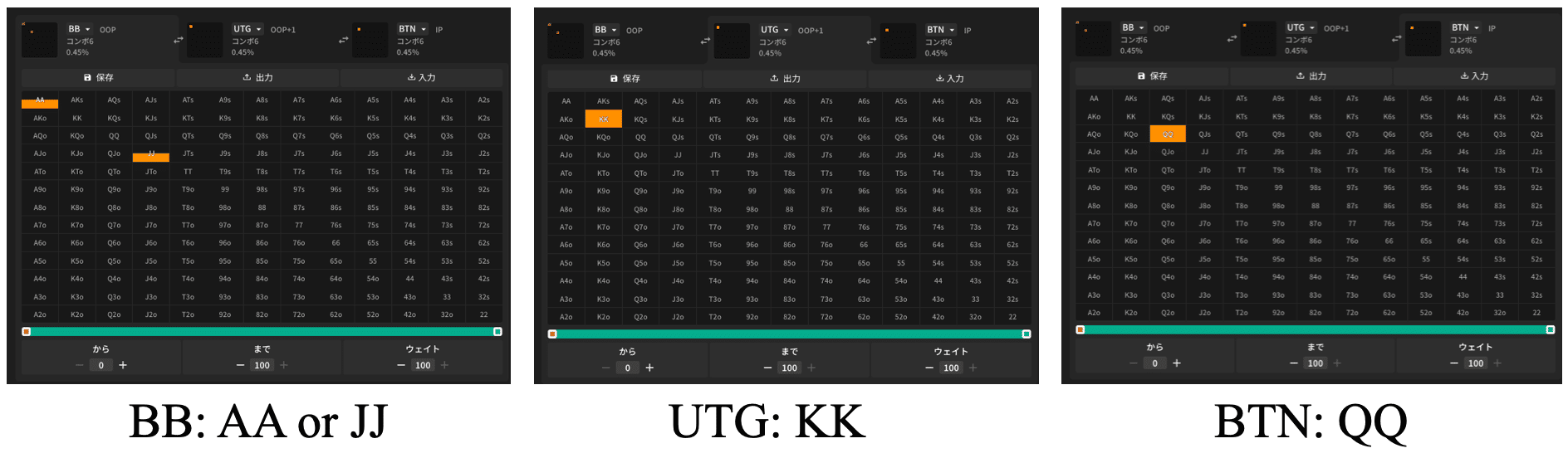
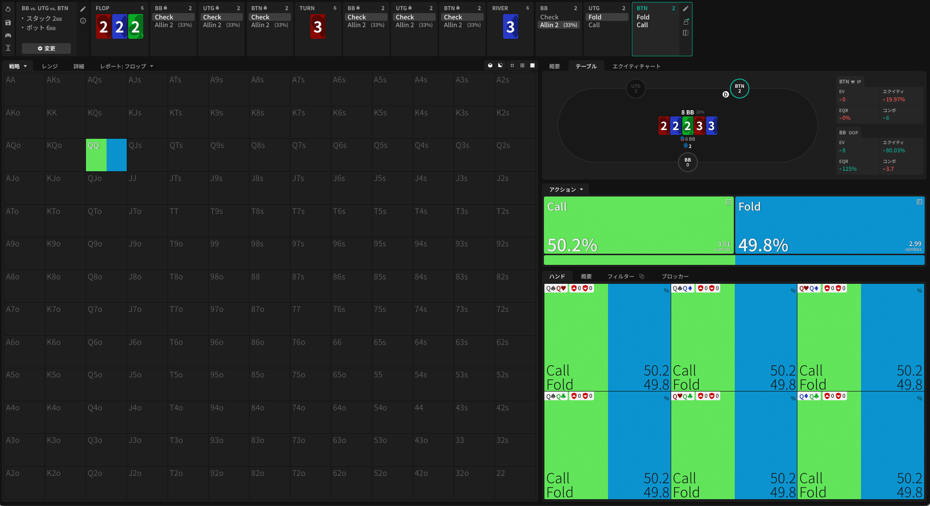
Finally, let us examine the AJ-K-Q game solution using GTO Wizard. We set up a 3-way with BB, UTG, and BTN, where BB holds AA and JJ with equal probability, UTG holds KK, and BTN holds QQ [Figure 5]. To examine only a 1-street river scenario, the board is set to 22233 (which cannot make a flush), and all flop and turn actions are nodelocked to pure check. The pot is 6bb, all players' stacks are 2bb, with no rake, and only all in (33% bet) is allowed as a river bet option.

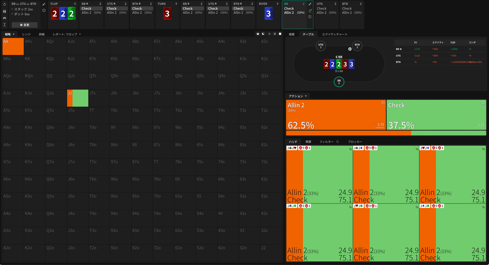
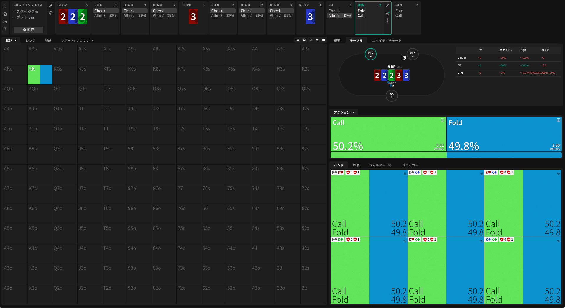
Figures 6–8 show each player's strategy on the river. First, BB pure bets AA and bets 25% of JJ while checking 75% [Figure 6]. The bet frequency of JJ equals alpha $${\alpha_{S=1/3}=\frac{1/3}{1+1/3}=\frac{1}{4}}$$ for a 33% bet size, matching the Nash equilibrium of the AJ-K-Q game described above. Against BB's all in (33% bet), UTG's KK is indifferent between calling and folding, calling 50% and folding 50% [Figure 7]. When UTG chooses to fold, BTN is similarly indifferent, with call and fold frequencies of 50% each [Figure 8]. The product of UTG and BTN's fold frequencies ($${0.5\times 0.5}$$) equals $${\alpha_{S=1/3}=0.25}$$, confirming that condition (1) holds and MDF sharing is taking place. Furthermore, note that the symmetric solution—where Players 2 and 3 (UTG and BTN) have equal fold frequencies—is selected among the Nash equilibria. As discussed in the previous section, the QRE actually outputs the symmetric solution that balances entropy.

Among the multiple existing Nash equilibria, from the perspective of MDF sharing regardless of which equilibrium is followed, each player must fold at a higher frequency than in a 2-player game. It is also interesting that the symmetric solution is endorsed both by the local stability analysis considering perturbations and by the Nash equilibrium as the limit of QRE (GTO Wizard's output). The symmetric solution can serve as a benchmark in the sense that it provides a typical fold frequency. That is, when two players share MDF, the fold frequency can be set to $${\sqrt{\alpha_S}}$$ for bet size $${S}$$. This result extends to $${N(\geq 2)}$$ players sharing MDF, where each of the $${N}$$ players should fold at $${\sqrt[N]{\alpha_S}}$$. This benchmark is also introduced in the Wizard blog.
[Note: In practice, results differ depending on catching hand strength and play order.]

Summary

• In this article, we examined two models—① the AJ-Q-K game and ② the AJ-K-Q game—to understand the fundamental properties of Nash equilibrium in multiway. These two models are natural extensions of the heads-up AKQ game, and it is confirmed that a player with a polarized range should bet value and bluffs at an appropriate ratio. The two models produce different Nash equilibria due to the different play order of two players holding catching hands of different strengths. In particular, in the AJ-K-Q game ②, the two players holding K and Q jointly create MDF by keeping the product of their individual fold frequencies constant.

• Nash equilibria generally exist in multiples, and in multiway, mixing strategies from different Nash equilibria to create a new strategy profile does not necessarily form a Nash equilibrium. Additionally, in multiway, Nash equilibrium loses its power to guarantee a minimum EV. These two points mean that strategies contained in multiway Nash equilibria cannot be considered GTO strategies with desirable properties.

• It was possible to discuss which among multiple Nash equilibria is closer to "optimal" by appropriately setting evaluation criteria. While various criteria exist, this article presented a method for selecting Nash equilibria based on the criterion of minimizing EV loss when perturbations are introduced around the equilibrium. This showed that the symmetric solution—where Players 2 and 3 have equal fold frequencies—is selected in the AJ-K-Q game.

• GTO Wizard outputs equilibrium solutions using QRE. In general, the Nash equilibria that arise as limits of QRE are restricted to only a subset of all possible Nash equilibria. The Nash equilibria selected in this way tend to maximize the entropy of each player's mixed strategy, and in the AJ-K-Q game, only the symmetric solution is selected. This result was confirmed by actually examining the solution using GTO Wizard.

Closing Remarks