Quantal Response Equilibrium (QRE) in the AKQ Game

Author: Sigma (Twitter: @sigm_4)

What You Will Learn

• What quantal response equilibrium (QRE) is

• How to concretely compute QRE (logit QRE; LQRE)

• How quantitatively different the QRE used in Wizard is from the conventional Nash equilibrium-based GTO strategy

• (For enthusiasts) In LQRE, the asymptotic behavior toward Nash equilibrium qualitatively differs depending on the nature of the hand

• (For enthusiasts) Through the correspondence with statistical mechanics, concepts such as entropy and free energy of mixed strategies can be applied, and LQRE can be formulated as a variational problem for the free energy

Introduction: Quantal Response Equilibrium (QRE)

What Is QRE?

Recently, GTO Wizard's introduction of Quantal Response Equilibrium (QRE) has become a hot topic (Japanese article, English article). Japanese commentary notes on QRE and ghost lines 👻 have also been written (by chin crypto (siguo), by Woody).

If you have read these notes or GTO Wizard's explanation, you may already understand what QRE is about. In this article, we start again from what QRE is, explain logit QRE as one computational model, and present an application to the most fundamental toy game: the AKQ game.

In simple terms, QRE is the equilibrium that arises when each player is not perfectly rational. Conventional Nash equilibrium-based GTO strategies relied on the strong assumption that perfectly rational players can accurately predict each other's actions. QRE accounts for the fact that players probabilistically make "mistakes" in their decision-making.

Several models exist for specifying what kinds of mistakes occur and with what probability, and the most representative among them is known as logit QRE (LQRE). As of the time of writing, GTO Wizard's explanation does not specify which QRE model is being used. Therefore, in this article, we take logit QRE as a plausible candidate and work through how the equilibrium is constructed, aiming to develop an intuitive understanding of QRE.

Representative Example: Logit QRE (LQRE)

In logit QRE (LQRE), the selection probability of each action is determined as an exponential function of that action's EV (given the opponent's strategy is fixed). That is, the probability that player $i$ takes action $a_i$ is:

$$ \begin{align*} P_i(a_i) = \frac{e^{\lambda\cdot\mathrm{EV}(a_i,P_{-i})}}{\sum_{a_i'}e^{\lambda\cdot\mathrm{EV}(a_i',P_{-i})}} \quad\quad (1) \end{align*} $$

Here, $P_{-i}$ denotes the mixed strategy profile of all players other than player $i$. $\mathrm{EV}(a_i,P_{-i})$ represents the expected payoff that player $i$ receives when taking action $a_i$ while the other players play the mixed strategy profile $P_{-i}$. The parameter $\lambda$ is a non-negative parameter called the rationality parameter.

Equation (1) states that as $\mathrm{EV}(a_i,P_{-i})$ increases, $P_i(a_i)$ increases exponentially. In other words, the player takes high-EV actions at high frequency (given the other players' mixed strategy profile is fixed). The key difference from Nash equilibrium is that the player does not exclusively choose the maximum-EV action at each node. So how much are suboptimal actions (actions other than the best action, i.e., the highest-EV action) considered? This is determined by the rationality parameter $\lambda$. The larger $\lambda$ is, the more it amplifies the exponent in equation (1), increasing the probability of choosing the best action. Conversely, for large $\lambda$, the probability of choosing any action other than the best drops sharply.

If we divide both the numerator and denominator of equation (1) by $e^{\lambda\cdot\mathrm{EV}(a_i^{\mathrm{best}},P_{-i})}$ corresponding to the best action $a_i^{\mathrm{best}}$, we get:

$$ \begin{align*} P_i(a_i) \sim e^{\lambda\cdot(\mathrm{EV}(a_i,P_{-i})-\mathrm{EV}(a_i^{\mathrm{best}},P_{-i}))} \end{align*} $$

From this, we can see that actions with EV roughly within $1/\lambda$ of the best action's EV are tolerated (have non-negligible probability). In the limit $\lambda\to\infty$, only the best action is tolerated, and the player becomes perfectly rational, yielding (a subset of) Nash equilibrium. On the other hand, in the limit $\lambda\to 0$, all actions are selected with equal weight, yielding the equilibrium for a completely irrational player.

To better understand the structure of LQRE, let us consider a simple concrete example. In a 1-street game, suppose (with the opponent's strategy fixed) the EV of betting with a certain hand is $\mathrm{EV}_{\mathrm{b}} = 2$ and the EV of checking is $\mathrm{EV}_{\mathrm{x}} = 1$. If we choose the rationality parameter $\lambda=1$, then by equation (1):

$$ \begin{align*} \text{Bet frequency} &= \frac{e^{1\cdot \mathrm{EV}_{\mathrm{b}}}}{e^{1\cdot \mathrm{EV}_{\mathrm{b}}} + e^{1\cdot \mathrm{EV}_{\mathrm{x}}}} \\ \text{Check frequency} &= \frac{e^{1\cdot \mathrm{EV}_{\mathrm{x}}}}{e^{1\cdot \mathrm{EV}_{\mathrm{b}}} + e^{1\cdot \mathrm{EV}_{\mathrm{x}}}} \end{align*} $$

The bet frequency is $e^{1\cdot(\mathrm{EV}_{\mathrm{b}}-\mathrm{EV}_{\mathrm{x}})}=e\simeq 2.7$ times higher than the check frequency. Now, assuming a more rational player with $\lambda=10$, the bet is selected $e^{10\cdot(\mathrm{EV}_{\mathrm{b}}-\mathrm{EV}_{\mathrm{x}})}=e^{10}\simeq 2.2\times 10^4$ times more frequently than the check. Since the EV difference between bet and check is 1, which is much larger than $1/\lambda=0.1$, the check option is almost never selected.

In general, the solution to LQRE is obtained through the following procedure. First, we assume some initial probabilities for all players' actions to fix their strategies, then determine the action probabilities according to equation (1) given those strategy profiles. Next, we require that these probabilities match the initially assumed probabilities. The probability distribution over all actions obtained in this self-consistent manner gives the LQRE solution. Algorithmically, the procedure is:

Assume probabilities for all players' actions (e.g., 50% bet / 50% check at this node, 30% call / 70% fold at that node)
→ Compute the right-hand side of equation (1) based on these assumptions to obtain new action probabilities
→ Use these new probabilities and equation (1) to obtain yet another set of probabilities
→ Repeat this procedure until the probability distribution converges
→ The converged result is the LQRE solution

To summarize:

• QRE describes the equilibrium among players who probabilistically make mistakes.

• LQRE, the most representative QRE model, is constructed so that the probability of selecting low-EV actions decays exponentially.

• In LQRE, the rationality parameter $\lambda$ controls how far below the best action's EV the model considers.

LQRE for the AKQ Game

In this section, we apply the LQRE introduced in the previous section to the well-known AKQ game to see what kind of equilibrium it produces.

Game Setup

The AKQ game is set up as follows:

- Player 1: Holds either A or Q with equal probability.
- Player 2: Holds K.
- Pot size: 1

- Only Player 1 can bet (or check) once (semi-street), with the bet size fixed at $B(>0)$ relative to the pot.
- Player 2 can call or fold against Player 1's bet; raising is not allowed.
- When Player 1 checks or Player 2 calls, a showdown occurs, and the player with the higher-ranking card wins the current pot.

Nash Equilibrium of the AKQ Game

Before looking at LQRE, let us review the Nash equilibrium of the AKQ game. The Nash equilibrium is:

- Player 1 always bets with A, and bets with Q at probability $\frac{B}{1+B}$ and checks at probability $\frac{1}{1+B}$.
- Player 2 calls Player 1's bet at probability $\frac{1}{1+B}$ and folds at probability $\frac{B}{1+B}$.

Player 1's bluff frequency with Q follows from the condition that makes Player 2's K indifferent between calling and folding. Player 2's call frequency with K follows from the condition that makes Player 1's Q indifferent between betting and checking.

LQRE of the AKQ Game and Interpretation

In LQRE, all actions are determined according to the probability distribution in equation (1). In the semi-street AKQ game, each hand has one action point, so we define:
- $p_{\mathrm{A}}$: Player 1's frequency of betting with A
- $p_{\mathrm{Q}}$: Player 1's frequency of betting with Q
- $p_{\mathrm{K}}$: Player 2's frequency of calling Player 1's bet with K

Under this probability distribution (mixed strategy), the EV that Player 1 obtains by betting with A is:

$$ \begin{align*} \mathrm{EV}_{\mathrm{A;\mathrm{b}}} = p_{\mathrm{K}}\cdot (1+B) + (1-p_{\mathrm{K}})\cdot 1 = 1+Bp_{\mathrm{K}} \end{align*} $$

Meanwhile, the EV from checking with A is:

$$ \begin{align*} \mathrm{EV}_{\mathrm{A;\mathrm{x}}} = 1 \end{align*} $$

Then, the probability that Player 1 bets with A, using equation (1), is:

$$ \begin{align*} \frac{e^{\lambda\cdot\mathrm{EV}_{\mathrm{A;\mathrm{b}}}}}{e^{\lambda\cdot \mathrm{EV}_{\mathrm{A;\mathrm{b}}}} + e^{\lambda\cdot \mathrm{EV}_{\mathrm{A;\mathrm{x}}}}} = \left(1 + e^{-\lambda Bp_{\mathrm{K}}}\right)^{-1} \end{align*} $$

Since we defined the probability of betting with A as $p_{\mathrm{A}}$:

$$ \begin{align*} p_{\mathrm{A}} = \left(1 + e^{-\lambda Bp_{\mathrm{K}}}\right)^{-1} \quad\quad (2) \end{align*} $$

Applying the same procedure to other actions using equation (1), we obtain:

$$ \begin{align*} p_{\mathrm{Q}} &= \left(1 + e^{-\lambda (1-(1+B)p_{\mathrm{K}})}\right)^{-1} \quad\quad (3) \\ p_{\mathrm{K}} &= \left(1 + e^{-\lambda \frac{-Bp_{\mathrm{A}}+(1+B)p_{\mathrm{Q}}}{p_{\mathrm{A}}+p_{\mathrm{Q}}}}\right)^{-1}  \quad\quad (4) \end{align*} $$

Solving the system of three simultaneous equations (2)-(4) yields the self-consistent probability distribution for all actions. In general, such nonlinear systems of equations are difficult to solve analytically and are typically solved numerically. Here, we performed numerical computation using Broyden's method (a type of quasi-Newton method). Figure 1 shows the numerically obtained LQRE solutions $p_{\mathrm{A}}, p_{\mathrm{Q}}, p_{\mathrm{K}}$ plotted as functions of $\lambda$ for several bet sizes $B =1/3, 1/2, 1, 2, 3$. The dashed lines indicate the Nash equilibrium values.

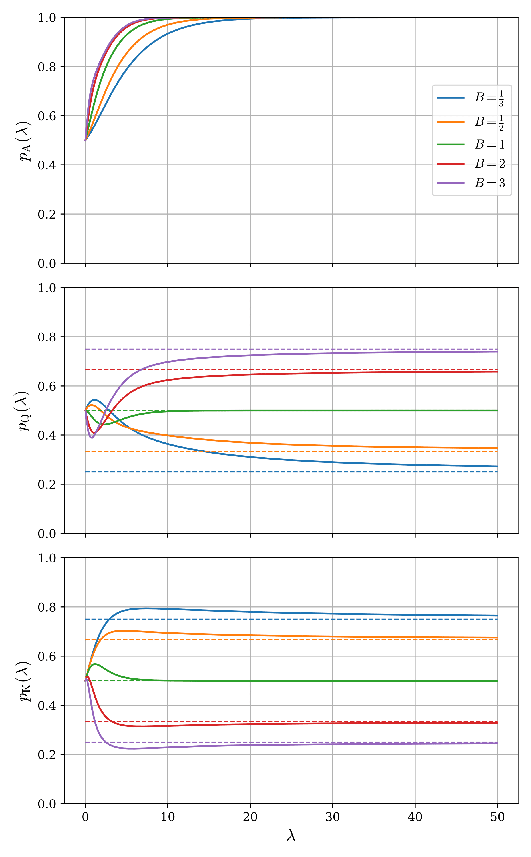
An immediate observation is that in the limit $\lambda\to 0$, all action frequencies equal 1/2, reproducing a completely irrational player (one who selects actions completely at random). On the other hand, in the limit $\lambda\to\infty$, the Nash equilibrium is recovered: Player 1's bet frequency with A approaches 1, the bet frequency with Q approaches $\frac{B}{1+B}$, and Player 2's call frequency with K approaches $\frac{1}{1+B}$. In the intermediate region, the behavior is non-monotonic and depends on $\lambda$. To understand these features, we examine below how the solutions behave when we deviate slightly from each limit (i.e., how they asymptotically approach the limiting values).

① When $\lambda$ is sufficiently small (completely irrational limit)
Expanding equations (2)-(4) under $\lambda\sim 0$ to first order in $\lambda$:

$$ \begin{align*} p_{\mathrm{A}} &\simeq \frac{1}{2}\left(1+\frac{Bp_{\mathrm{K}}}{2}\lambda\right) \\ p_{\mathrm{Q}} &\simeq \frac{1}{2}\left(1+\frac{1-(1+B)p_{\mathrm{K}}}{2}\lambda\right) \\ p_{\mathrm{K}} &\simeq \frac{1}{2}\left(1+\frac{-Bp_{\mathrm{A}}+(1+B)p_{\mathrm{Q}}}{2(p_{\mathrm{A}}+p_{\mathrm{Q}})}\lambda\right) \end{align*} $$

Solving these gives:

$$ \begin{align*} p_{\mathrm{A}} &\simeq \frac{1}{2}\left(1+\frac{B}{4}\lambda\right) \\ p_{\mathrm{Q}} &\simeq \frac{1}{2}\left(1+\frac{1-B}{4}\lambda\right) \\ p_{\mathrm{K}} &\simeq \frac{1}{2}\left(1+\frac{1}{4}\lambda\right) \end{align*} $$

Indeed, in Figure 1 we can see that $p_{\mathrm{A}}$ and $p_{\mathrm{K}}$ rise with a positive slope near $\lambda\sim 0$, while $p_{\mathrm{Q}}$ rises with a positive slope when the bet size is less than 1 and a negative slope when it is greater than 1. This result can be interpreted as follows: Player 1, who was completely irrational, gains a slight degree of rationality and realizes they have been betting their strong A far too infrequently. Furthermore, considering MDF, they notice that when the bet size exceeds 1 the opponent is overcalling, and when it is less than 1 the opponent is overfolding. Accordingly, they decide to bluff less when the bet size exceeds 1 and bluff more when it is less than 1. Player 2 similarly gains a slight degree of rationality and notices that the opponent's value-to-bluff ratio is 1:1 regardless of bet size, meaning the opponent is always bluffing too much relative to MDF, so they decide to increase their call frequency.

② When $\lambda$ is sufficiently large (completely rational limit)
We expand equations (2)-(4) under the assumption that $\lambda$ is sufficiently large. For each action probability $p_{\mathrm{X}}\,(\mathrm{X}=\mathrm{A}, \mathrm{K}, \mathrm{Q})$, we denote the Nash equilibrium value with a $^*$ superscript and write:

$$ \begin{align*} p_{\mathrm{X}} &= p_{\mathrm{X}}^* + \delta p_{\mathrm{X}} \end{align*} $$

where $\delta p_{\mathrm{X}}$ is $\omicron(1)$ (using Landau's notation, $f(\lambda)$ is $\omicron(g(\lambda))$ if $\frac{f(\lambda)}{g(\lambda)}\to 0$ as $\lambda\to\infty$).

From equation (2) and $p_{\mathrm{A}}^*=1,  p_{\mathrm{K}}^*=\frac{1}{1+B}$:

$$ \begin{align*} \delta p_{\mathrm{A}} = -\frac{e^{-(\lambda\frac{B}{1+B}+\lambda B \delta p_{\mathrm{K}})}}{1+e^{-(\lambda\frac{B}{1+B}+\lambda B \delta p_{\mathrm{K}})}} = -e^{-(\lambda\frac{B}{1+B}+\lambda B \delta p_{\mathrm{K}})} + \omicron(e^{-\lambda\frac{B}{1+B}}) \end{align*} $$

From equation (3) and $p_{\mathrm{Q}}^*=\frac{B}{1+B},  p_{\mathrm{K}}^*=\frac{1}{1+B}$:

$$ \begin{align*} \delta p_{\mathrm{Q}} = \frac{1}{1+e^{\lambda(1+B)\delta p_{\mathrm{K}}}} - \frac{B}{1+B} \end{align*} $$

For the right-hand side to be $\omicron(1)$, we need $e^{\lambda(1+B)\delta p_{\mathrm{K}}}\to 1/B$, which gives:

$$ \begin{align*} \delta p_{\mathrm{K}} = -\frac{\ln B}{1+B}\frac{1}{\lambda} + \omicron(\lambda ^{-1}) \end{align*} $$

Finally, from equation (4):

$$ \begin{align*} \delta p_{\mathrm{K}} = \frac{1}{1+e^{-\lambda\frac{-Bp_{\mathrm{A}}+(1+B)p_{\mathrm{Q}}}{p_{\mathrm{A}}+p_{\mathrm{Q}}}}} - \frac{1}{1+B} \end{align*} $$

For the right-hand side to be $\omicron(1)$, noting that:

$$ \begin{align*} \frac{-Bp_{\mathrm{A}}+(1+B)p_{\mathrm{Q}}}{p_{\mathrm{A}}+p_{\mathrm{Q}}} &= \frac{-B\delta p_{\mathrm{A}}+(1+B)\delta p_{\mathrm{Q}}}{p_{\mathrm{A}}^*+p_{\mathrm{Q}}^*} + \omicron(\lambda^{-1}) \\ &= \frac{1+B}{1+2B}(-B\delta p_{\mathrm{A}}+(1+B)\delta p_{\mathrm{Q}}) + \omicron(\lambda^{-1}) \end{align*} $$

we obtain:

$$ \begin{align*} \delta p_{\mathrm{Q}} = -\frac{1+2B}{(1+B)^2}\ln B\cdot\frac{1}{\lambda} + \omicron(\lambda^{-1}) \end{align*} $$

Collecting the final results:

$$ \begin{align*} p_{\mathrm{A}} &= 1 - \left(\frac{1}{B}\right)^{\frac{B}{1+B}}e^{-\frac{B}{1+B}\lambda} + \omicron(e^{-\frac{B}{1+B}\lambda}) \quad\quad (5) \\ p_{\mathrm{Q}} &= \frac{B}{1+B} - \frac{1+2B}{(1+B)^2}\ln B\cdot\frac{1}{\lambda} + \omicron(\lambda^{-1}) \quad\quad (6) \\ p_{\mathrm{K}} &= \frac{1}{1+B} - \frac{\ln B}{1+B}\frac{1}{\lambda} + \omicron(\lambda^{-1}) \quad\quad (7) \end{align*} $$

A notable point is that $p_{\mathrm{A}}$ approaches its limiting value exponentially in $\lambda$. While $p_{\mathrm{Q}}$ and $p_{\mathrm{K}}$ converge slowly as powers of $\lambda^{-1}$, $p_{\mathrm{A}}$ converges rapidly with increasing player rationality. Furthermore, since the exponent $\frac{B}{1+B}$ is monotonically increasing in $B$, larger bet sizes lead to even faster asymptotic convergence. Looking at Figure 1, we can indeed confirm that $p_{\mathrm{A}}$ locks onto its limiting value much more rapidly than the others, and the bet size dependence is also visible. Since there is no check frequency for A in Nash equilibrium, we can say that checking with A is strongly "forbidden" by rationality. It is highly interesting that the fact that one action's EV exceeds the others at Nash equilibrium is not merely reflected in the selection probabilities under LQRE, but also produces a qualitative difference in the behavior with respect to rationality.

As a minor note, let us add a remark about the case $B=1$. As can be seen from equations (6) and (7), when $B=1$ the coefficient of $\lambda^{-1}$ for both $p_{\mathrm{Q}}$ and $p_{\mathrm{K}}$ vanishes. Although we omit the detailed calculation here, when $B=1$ the asymptotic forms of $p_{\mathrm{Q}}$ and $p_{\mathrm{K}}$ as $\lambda\to\infty$ are in fact no longer power-law but exponential. As can be read from Figure 1, they approach their limiting value of $1/2$ extremely rapidly. This exponential behavior can in some sense be called critical, representing an "anomalous" phenomenon occurring at a special value.

Next, focusing on the coefficient of $\lambda^{-1}$ in $p_{\mathrm{Q}}$ and $p_{\mathrm{K}}$, we can see that when the bet size is greater/less than 1, they approach their limiting values from below/above, respectively. This can indeed be read from Figure 1. This fact can be interpreted as follows. Two formerly perfectly rational players begin to make mistakes as they each lose a slight degree of rationality. When Player 1 bluff-bets (bets with Q), they feel more risk when the bet size is large and reduce their bluff frequency, while feeling less risk when the bet size is small and increasing their bluff frequency. In response, Player 2 perceives the call EV as lower than fold EV when the bet size is large and higher when it is small (as a result, in Nash equilibrium the call frequency and fold frequency reverse at $B=1$). Conversely, when Player 2 calls with K, they likewise feel more risk when the bet size is large and reduce their call frequency, while feeling less risk when the bet size is small and increasing their call frequency. In response, Player 1 perceives Q's bluff-bet EV as higher than check EV when the bet size is large and lower when it is small (as a result, in Nash equilibrium Q's bluff-bet frequency and check frequency reverse at $B=1$).

Exploitability of LQRE

In this section, we evaluate the accuracy of LQRE. A well-known metric for how much a strategy can be exploited is exploitability (= Nash distance). Exploitability measures how much EV a strategy loses compared to what the GTO strategy guarantees when facing the maximally exploitative strategy (MES) against it.

Below, we estimate Player 1's exploitability $\varepsilon$. When Player 1's value-to-bluff ratio under LQRE is more value-heavy than the Nash equilibrium ratio, the MES for Player 2 is to always fold K. Conversely, when Player 1's betting is bluff-heavy, the MES for Player 2 is to always call with K. With this in mind:

- In the bluff-heavy case, Player 1's strategy EV is $\frac{1}{2} + \frac{B}{2}(p_{\mathrm{A}} - p_{\mathrm{Q}})$
- In the value-heavy case, Player 1's strategy EV is $\frac{1}{2}(1+p_{\mathrm{Q}})$

Since Player 1's EV under the GTO strategy is $\frac{1+2B}{2(1+B)}$, subtracting the EV obtained when facing the MES gives:

$$ \begin{align*} \varepsilon = \begin{cases} \frac{B}{2(1+B)} - \frac{B}{2}(p_{\mathrm{A}} + p_{\mathrm{Q}}) & \text{if bluff-heavy} \\ \frac{B}{2(1+B)} - \frac{p_{\mathrm{Q}}}{2} &\text{if value-heavy} \end{cases} \quad\quad (8) \end{align*} $$

Figure 2 plots the exploitability as a function of $\lambda$ using the numerically obtained LQRE results. As $\lambda$ increases, LQRE approaches Nash equilibrium and the exploitability converges to 0.

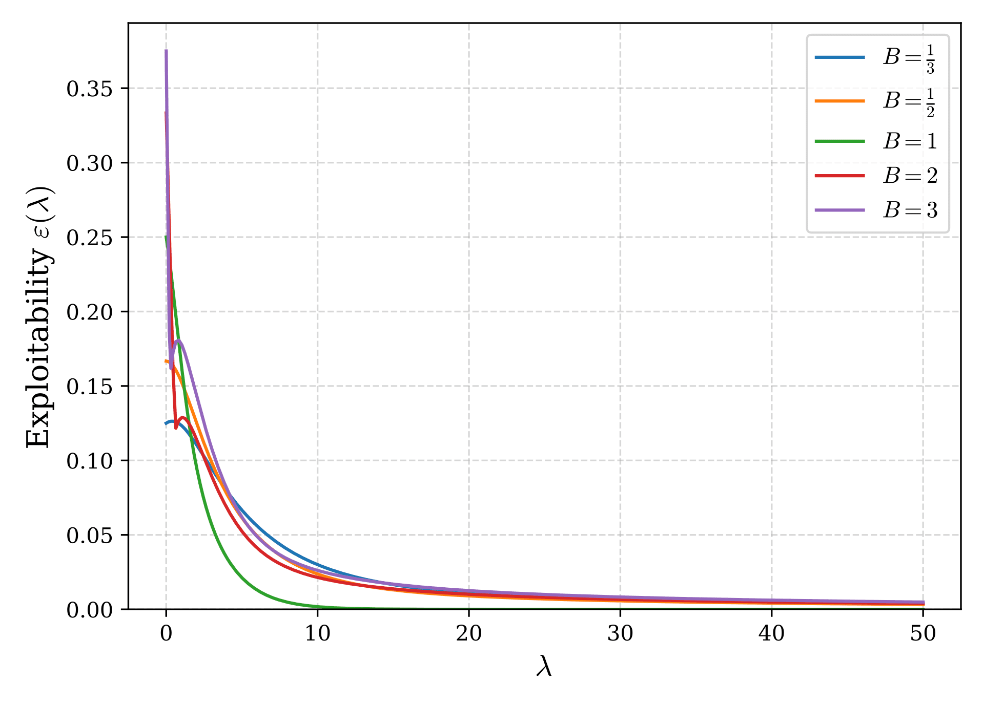
To investigate how large $\lambda$ must be for the exploitability to become sufficiently small, we evaluate $\varepsilon$ using the asymptotic solutions derived earlier for $\lambda\to\infty$. Substituting equations (5) and (6) into equation (8), we obtain as $\lambda\to\infty$:

$$ \begin{align*} \varepsilon(\lambda) &=\begin{cases} -\frac{\delta p_{\mathrm{Q}}}{2}& \text{if } B >1 \\ -\frac{B}{2}(\delta p_{\mathrm{A}} - \delta p_{\mathrm{Q}}) & \text{if } B <1 \end{cases} \\ &= \begin{cases} \frac{1+2B}{2(1+B)^2}\ln B\cdot\frac{1}{\lambda} + \omicron(\lambda^{-1})& \text{if } B >1 \\ -\frac{B(1+2B)}{2(1+B)^2}\ln B\cdot\frac{1}{\lambda} + \omicron(\lambda^{-1}) & \text{if } B <1 \end{cases} \end{align*} $$

Here, the case distinction arises because for sufficiently large $\lambda$, $B\gtrless 1$ corresponds to value-heavy and bluff-heavy, respectively (see the earlier discussion). The important point is that the leading order of exploitability is $\Omicron(\lambda^{-1})$ (using Landau's notation, $f(\lambda)$ is $\Omicron(g(\lambda))$ if $\frac{f(\lambda)}{g(\lambda)}\to \mathrm{const.}$ as $\lambda\to\infty$). This originates from the asymptotic form of $p_{\mathrm{Q}}$. Although $p_{\mathrm{A}}$ converges exponentially, the exploitability accounts for all hands and thus picks up the slowest-converging $\Omicron(\lambda^{-1})$ term from $p_{\mathrm{Q}}$.

For example, when $B=2$ or $B=1/2$, the coefficient of $1/\lambda$ is $\frac{5\ln2}{18}\simeq 0.1925$ and $\frac{2\ln2}{9}\simeq 0.1540$, respectively. In either case, choosing $\lambda = 2000$ or so is expected to keep the exploitability below 0.1% of the pot. The 0.1% figure is mentioned in the GTO Wizard blog:

GTO Wizard AI converges its solutions to a Nash distance where they can only be exploited for approximately 0.1% of the pot size.

When $\lambda = 2000$, as can be seen from equations (5)-(7), $p_{\mathrm{A}}$ is extremely close to 1, while $p_{\mathrm{Q}}$ and $p_{\mathrm{K}}$ deviate from their Nash equilibrium values by only about 0.1%. One could say this is approximately Nash equilibrium to 99.9% accuracy (this is also called an $\varepsilon$-equilibrium). In other words, the QRE recently introduced to GTO Wizard is virtually identical to the Nash equilibrium-based GTO strategies we have been using.

[Note: There is a meaningful change in that nodes where the transition probability was zero and computation had not converged under the previous GTO Wizard (so-called ghost lines) have been improved. However, since those transition probabilities are themselves negligibly low in practice, it is fair to say that QRE is essentially the same as the previous Nash equilibrium-based GTO strategy. That said, when multiple Nash equilibria exist, the $\varepsilon$-equilibrium found by CFR and the $\varepsilon$-equilibrium from QRE could differ (be strategically distant from each other).]

Summary

• QRE describes the equilibrium among players who probabilistically make mistakes, and LQRE is its most representative model. In LQRE, the rationality parameter $\lambda$ controls how far below the best action's EV the model considers.

• In this article, we numerically solved LQRE for the AKQ game. The two limits $\lambda\to 0$ and $\lambda\to\infty$, and the manner of asymptotic approach, can be studied analytically.

• In particular, as $\lambda\to\infty$, LQRE approaches Nash equilibrium. A, which should adopt a pure strategy at Nash equilibrium, converges exponentially fast, while other hands that adopt mixed strategies converge slowly as power laws.

• The exploitability of LQRE, rate-limited by the power-law convergence of hands other than A, converges to 0 proportionally to $1/\lambda$.

• For the AKQ game, we concretely confirmed that setting $\lambda\approx 2000$ keeps the exploitability below 0.1% of the pot. At this point, the probability distribution of each action differs from Nash equilibrium by only about 0.1%.

Supplement: Statistical Mechanics Analogy

Correspondence with Statistical Mechanics

LQRE has a deep connection to statistical mechanics in physics. The probability distribution in equation (1), which forms the backbone of LQRE, is known in statistical mechanics as the Boltzmann distribution. The Boltzmann distribution describes the energy distribution of a classical particle ensemble (a collection of particles obeying classical, not quantum, mechanics), where the probability of the ensemble being in state $i$ with energy $\epsilon_i$ is given by:

$$ \begin{align*} \frac{e^{-\beta\epsilon_i}}{\sum_j e^{-\beta\epsilon_j}} \quad\quad (9) \end{align*} $$

Here, $\beta$ represents the reciprocal of temperature and is called the inverse temperature. Comparing equations (1) and (9), we can identify the following correspondence:

$$ \begin{align*} \epsilon_i &= - \mathrm{EV}(a_i,P_{-i}) \quad\quad (10) \\ \beta &= \lambda \quad\quad (11) \end{align*} $$

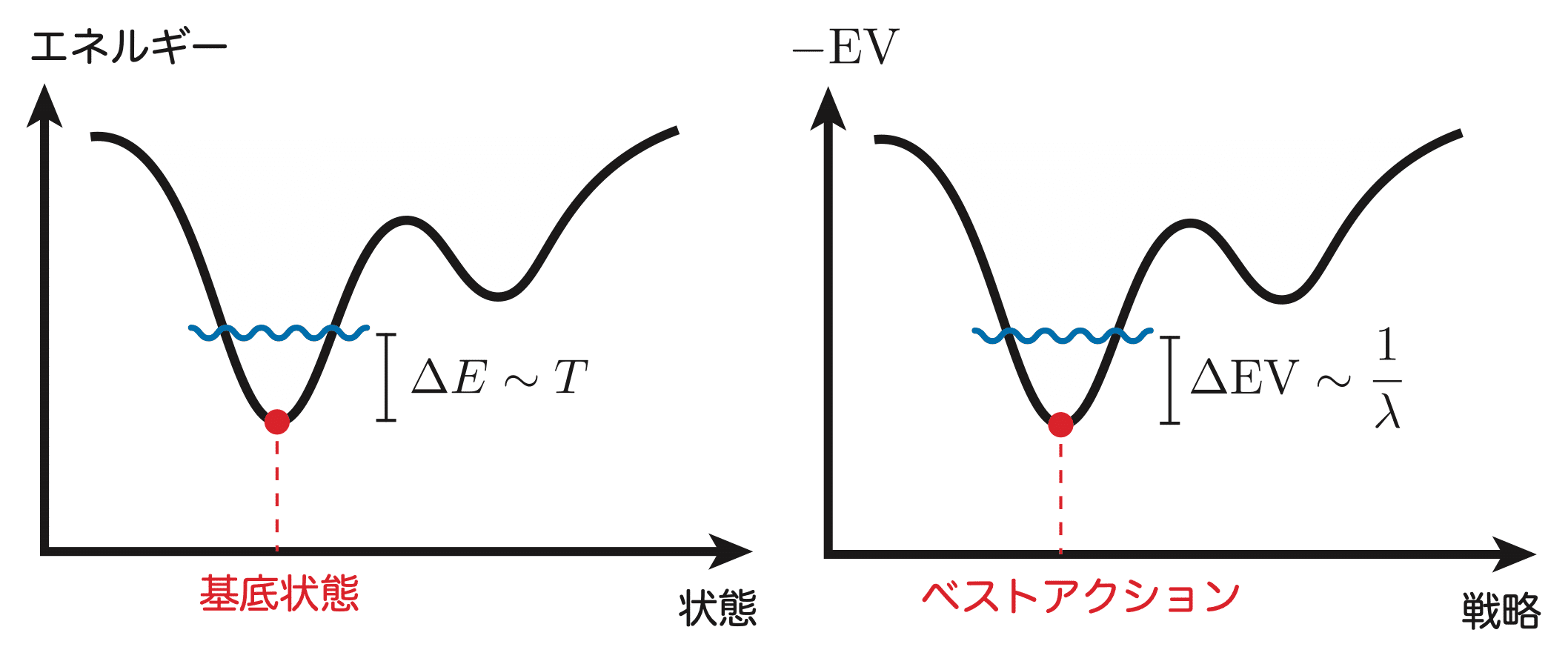
The negative sign in equation (10) arises because in poker (and game theory) the expected payoff is maximized, whereas in physics lower-energy states are preferred. Equation (11) indicates that $1/\lambda$ corresponds to the temperature $T$. In physics, at absolute zero ($T=0$), only the lowest-energy state (called the ground state) is realized, corresponding to the completely rational limit $\lambda\to\infty$ where only the maximum-EV action is realized at Nash equilibrium. At finite temperature, the particle ensemble does not only occupy the lowest-energy state but permits excitations (transitions to higher-energy states) on the order of the temperature $T$. In the high-temperature limit ($T\to\infty$), the ensemble occupies all states, corresponding to the completely irrational limit $\lambda\to 0$ in LQRE.

Figure 3 illustrates the correspondence between statistical mechanics (left) and LQRE (right). Just as thermal fluctuations at finite temperature allow excitations from the ground state to higher-energy states, in LQRE, actions with EV roughly $1/\lambda$ below the best action (the highest-EV action) are taken into account.

Considering this correspondence, LQRE in poker (or more generally in game theory) can be said to describe the strategy distribution in thermal equilibrium at temperature $1/\lambda$. This allows us to define various state quantities and thermodynamic functions for poker. For example, the entropy $S(P_i,P_{-i})$ of player $i$'s mixed strategy $P_i$ can be defined as:

$$ \begin{align*} S(P_i,P_{-i}) = - \sum_{a_i} P_i(a_i)\ln P_i(a_i) \end{align*} $$

where $P_i(a_i)$ is the LQRE probability distribution defined by equation (1). In physics, entropy serves as a measure of the disorder of a system. In poker (or game theory), it represents the randomness of the mixed strategy. It can also be described as a measure of how "uncertain" or how much "information content" the mixed strategy has. Using entropy, we can further define the Helmholtz free energy $F(P_i,P_{-i})$:

$$ \begin{align*} F(P_i,P_{-i}) = E(P_i,P_{-i}) - \frac{1}{\lambda}S(P_i,P_{-i}) \quad\quad (12) \end{align*} $$

where

$$ \begin{align*} {E(P_i,P_{-i})=-\sum_{a_i}P_i(a_i)\cdot\mathrm{EV}(a_i,P_{-i})} \quad\quad (13) \end{align*} $$

is called the internal energy, representing the EV at a given node. In physics, the free energy is roughly the energy that can be extracted as work, and it is a function that characterizes the stability of the system. A system naturally evolves to minimize its free energy, reaching thermal equilibrium. That is, at thermal equilibrium, the free energy takes its minimum value.

In fact, LQRE can also be formulated as a variational problem for the free energy. Below, instead of taking the specific form of the probability distribution in equation (1) as given, we derive equation (1) from the condition that the free energy in equation (12) should be minimized at thermal equilibrium. To do this, we consider the constraint on the probability distribution:

$$ \begin{align*} \sum_{a_i} P_i(a_i) = 1 \end{align*} $$

Introducing a Lagrange multiplier $\mu$, we define the functional:

$$ \begin{align*} \mathcal{F}[P_i] = F(P_i,P_{-i}) + \mu\left(\sum_{a_i}P_i(a_i)-1\right) \end{align*} $$

The functional derivative of $\mathcal{F}[P_i]$ must vanish:

$$ \begin{align*} \frac{\delta\mathcal{F}}{\delta P_i(a_i)} = 0 \end{align*} $$

This holds at thermal equilibrium. Performing the functional derivative using the expressions in equations (12) and (13):

$$ \begin{align*} -\mathrm{EV}(a_i,P_{-i}) - \frac{1}{\lambda}(1 + \ln P_i(a_i)) + \mu = 0 \end{align*} $$

Solving for $P_i(a_i)$:

$$ \begin{align*} P_i(a_i) = (\mathrm{const}.)\times e^{\lambda\cdot\mathrm{EV}(a_i,P_{-i})} \end{align*} $$

Normalizing this gives:

$$ \begin{align*} P_i(a_i) = \frac{e^{\lambda\cdot\mathrm{EV}(a_i,P_{-i})}}{\sum_{a_i'}e^{\lambda\cdot\mathrm{EV}(a_i',P_{-i})}} \end{align*} $$

which is precisely the LQRE probability distribution of equation (1).

Internal Energy, Entropy, and Free Energy of Mixed Strategies

In this final section, we present computational results for the state quantities and thermodynamic functions introduced in the statistical mechanics correspondence section: internal energy, entropy, and free energy. Recall that internal energy is the EV with a sign change, entropy indicates how much the mixed strategy mixes various actions, and free energy serves as a stability measure of the mixed strategy.

Figure 4 plots the internal energy $E_{\mathrm{X}}$, entropy $S_{\mathrm{X}}$, and free energy $F_{\mathrm{X}}$ for each hand as functions of $\lambda$, where ${\mathrm{X}} = \mathrm{A}, \mathrm{Q}, \mathrm{K}$, with each hand shown in a separate column.

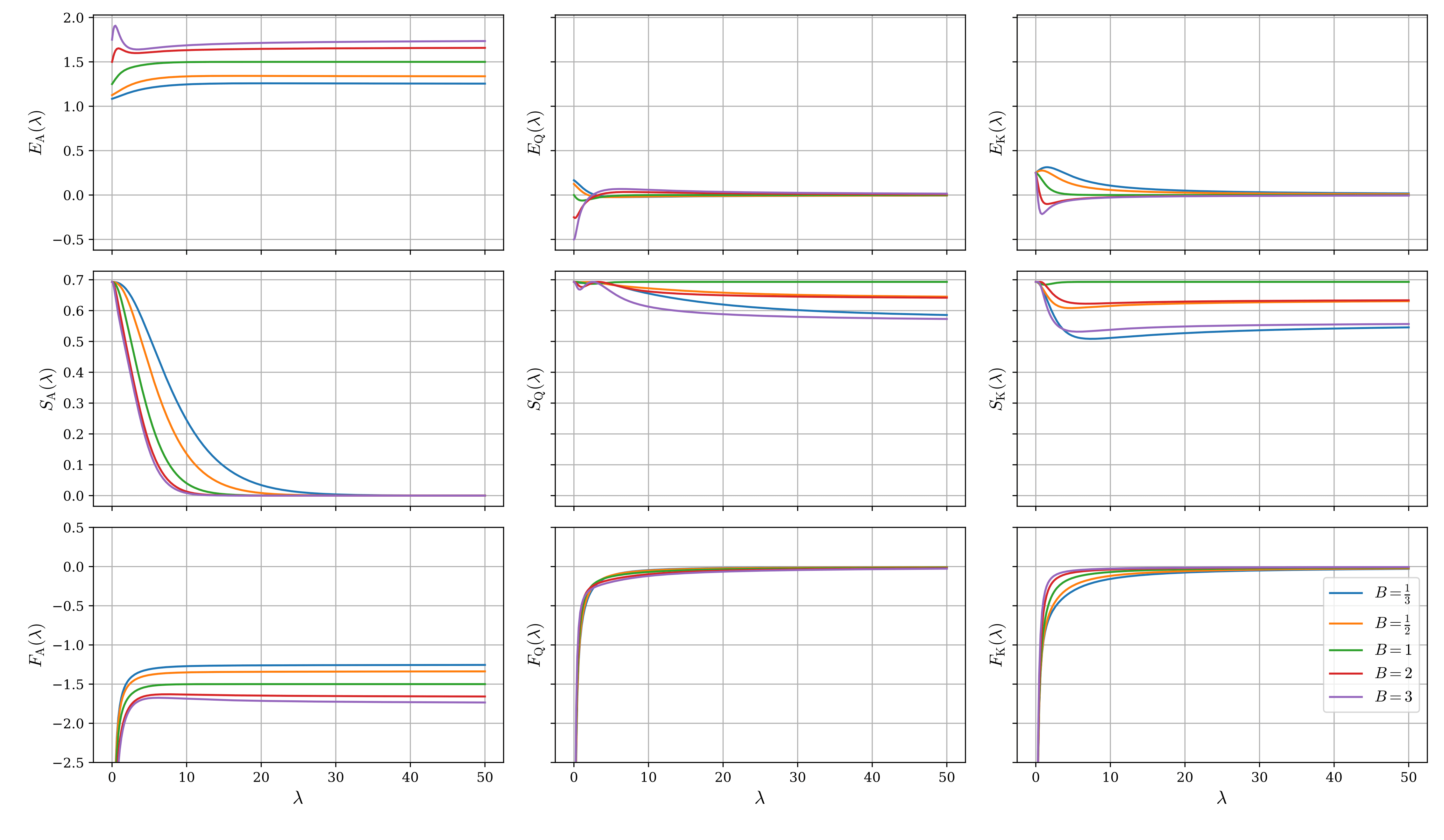
In the limit $\lambda\to 0$, all actions occur with equal probability, forming a completely random mixed strategy. Therefore, the entropy takes its maximum value of $\ln 2$. Since Player 1's A adopts a pure strategy (bet only) at Nash equilibrium, the entropy converges to its minimum value of 0 in the limit $\lambda\to\infty$. For the other hands, since they remain mixed strategies even at Nash equilibrium, the entropy settles to finite values.

The free energy is $F_{\mathrm{X}} = E_{\mathrm{X}} - \frac{1}{\lambda}S_{\mathrm{X}}$. As $\lambda$ increases, the entropy term (the second term) contributes less and less, and the free energy converges to the internal energy. As discussed above, since LQRE is obtained by choosing the probability distribution that minimizes the free energy, a rational player determines their strategy to maximize EV (which is the internal energy with a sign change). Conversely, as $\lambda$ decreases, the entropy term becomes increasingly significant, so making the mixed strategy as random as possible (maximizing entropy) works in the direction of reducing the free energy.

Closing Remarks