Hypergeometric Size: Bet Sizing When Your Opponent Has Draw Outs

Author: Sigma (Twitter: @sigm_4)

1. Introduction: More than geometric? Less than geometric?

It is common knowledge that on static boards, when your range contains nuttish hands, a polarized strategy using geometric sizing can be employed. But what happens when the board becomes dynamic—should you use a size larger than geometric, or smaller?

Some might answer smaller. Their reasoning could be that since your opponent's draw hands might overtake you on later streets, it is risky to build the pot with a size that commits you to going all in.
Others might answer larger. Their reasoning could be that by making a large bet that gives your opponent's draw hands unfavorable odds to call, you can achieve equity denial against those hands.

Thus, there are incentives to adjust the bet size in both directions. However, in practice, very few players intentionally use a size larger than geometric (= hypergeometric size).
In this article, we will deepen our understanding of bet size selection—particularly hypergeometric size—when your opponent has draw outs, through model calculations.

Following the model calculations in Chapter 2 requires some familiarity with computing GTO solutions for the AKQ model (and its variants) as well as the underlying mathematical procedures, so some readers may find it challenging.
In that case, feel free to skip ahead to Chapter 3, where we compare the model results with actual spots where hypergeometric size is used.

2. Model Calculations

2.1. First Model: "Pseudodynamic" 2-Street AKQ Model

To begin, consider the following 2-street AKQ model with draw outs and variable bet sizing.

OOP: A or Q (dealt with equal probability)
IP: K
・SPR: $S$
・Betting is allowed across 2 streets (referred to as the turn and river respectively).
・On the river, either K or 2 is revealed as a community card (with probabilities $p$ and $1-p$ respectively, where $p$ is assumed to be sufficiently small).
・Raising is prohibited (not strictly necessary but simplifies the discussion).
・Bet size: $r\in[0,S]$ on the turn, $r'\in[0,S']$ on the river (where $S'$ is the SPR at the start of the river).

We assume the following GTO strategy for this model.

Turn
・OOP: Bets A as a pure bet, and bets Q at frequency $x$, where $x\in[0,1]$ is set to make IP's K indifferent between calling and folding.
・IP: K is indifferent between calling and folding.

River (after a turn bet→call sequence)
・OOP: If K is dealt on the river, OOP range checks. If 2 is dealt, OOP pure bets A and bets Q at frequency $\frac{r'}{1+r'}=:\alpha'$ (making IP's K indifferent).
・IP: If 2 is dealt, K is indifferent between calling and folding against the bet.

IP's K call frequency (fold frequency) is determined by the condition that makes OOP's Q indifferent between betting and checking, but since it does not affect the following discussion, we omit it.

Using the fact that IP's K is indifferent between calling and folding against the turn bet, we can compute OOP's EV as if K always folds:

$$ \begin{align*} \mathrm{EV}_{\mathrm{OOP}}=(\text{OOP's turn bet frequency})\times (\text{Pot size})=\frac{1+x}{2}\times 1 \end{align*} $$

Therefore, we can calculate EV by finding Q's bet frequency $x$.
From the condition that IP's K is indifferent between calling and folding against the turn bet:

$$ \begin{align*} &(\text{K's Fold EV}) = (\text{K's Call EV}) \\ \Leftrightarrow {}& 0 = -r + p(1+2r)+(1-p)\frac{\frac{1}{2}(x-\alpha')}{\frac{1}{2}(1+x)}(1+2r)\quad\quad(1) \end{align*} $$

The first term on the right-hand side is the amount required to call the turn bet. The second term corresponds to the case where K is dealt on the river: $(\text{probability K is dealt})\times(\text{IP's EV when K is dealt}[=\text{Pot size}])$. The third term corresponds to the case where 2 is dealt on the river: $(\text{probability 2 is dealt})\times(\text{IP's EV when 2 is dealt}[=(\text{probability OOP checks})\times(\text{Pot size})])$.

Here we implicitly assume that OOP's check probability on the river is positive. That is, we impose:

$$ \begin{align*} x\geq\alpha' \end{align*} $$

Solving equation (1) yields:

$$ \begin{align*} x=(1-p)(\alpha'+(1+\alpha')\alpha)-p \quad\quad(2) \end{align*} $$

where $\alpha:=\frac{r}{1+r}$ is the alpha corresponding to bet size $r$.

In particular, when $p=0$ (i.e., 2 is always dealt on the river), we get $x=\alpha'+(1+\alpha')\alpha$, recovering the standard static 2-street AKQ model result. In this case, OOP bets the river bluff (Q) frequency $\alpha'$ plus, on the turn, the alpha that would apply if all hands that bet on the river were value hands ($=(1+\alpha')\alpha$).

Looking at equation (2), the bluff frequency $x$ in the dynamic case takes the form of a correction applied to the static case. The first term of equation (2) corrects the static bluff frequency by multiplying it by the probability that 2 is dealt on the river. The second term reduces the bluff frequency to account for the possibility that K is dealt on the river.

We can maximize OOP's EV by varying $r$ and $r'$ to maximize $x$. Since the first term of equation (2) corresponds to the bluff frequency in the static case ($p=0$), the well-known result for the static 2-street AKQ model gives us:

$$ \begin{align*} r=r'=\frac{-1+\sqrt{1+2S}}{2} \end{align*} $$

as the values that maximize $x$.

Therefore, even though this model considers a dynamic situation where the opponent has draw outs, it yields a result that affirms geometric sizing, just as in the static case. This is because the symmetry between turn and river bet sizes is not broken.
Moreover, in this model, when the draw completes (K is dealt), IP wins outright and no meaningful betting occurs for either player. When the river card is a rag (2 is dealt), both players' range equities are preserved. This makes it a "pseudodynamic" model. Therefore, below we consider an alternative model that introduces modifications to create a truly dynamic situation.

2.2. Second Model: Dynamic 2-Street AKQ Model

As our new model, we consider the following 2-street model with draw outs and variable bet sizing.

OOP: A or 2 (dealt with equal probability)
IP: $X_1, X_2, \cdots, X_N$ (dealt with equal probability)
・$\{X_i\}$ are distinct hands that are weaker than A but stronger than 2. For $N=4$, think of something like $X_1=K, X_2=Q, X_3=J, X_4=T$.
・SPR: $S$
・Betting is allowed across 2 streets (referred to as the turn and river respectively).
・On the river, elements from ${\{X_i|i=1, \cdots,N}\}$ appear uniformly.
・Raising is allowed.
・Bet size: $r\in[0,S]$ on the turn, $r'\in[0,S']$ on the river (where $S'$ is the SPR at the start of the river).

In this model, $\frac{1}{N}$ of IP's range completes a draw on the river and gets promoted to the nuts, while the remaining $\frac{N-1}{N}$ maintain their strength between OOP's A and 2. We assume $N$ is sufficiently large and posit the following GTO strategy for this model.

Turn
・OOP: Bets A as a pure bet, and bets 2 at frequency $x$, where $x\in[0,1]$ is set to make IP's $\{X_i\}$ indifferent between calling and folding.
・IP: All $\{X_i\}$ are indifferent between calling and folding.

River (after a turn bet→call sequence, river card $X_j$)
・OOP: Pure bets A, bets 2 at frequency $\frac{r'}{1+r'}=:\alpha'$ (making IP's $\{X_i|i\neq j\}$ indifferent).
・IP: Against the bet, $X_j$ pure raises all in, $\{X_i|i\neq j\}$ raise at an appropriate frequency, and the rest call or fold at appropriate frequencies.

From the condition that IP's $\{X_i\}$ are indifferent between calling and folding on the turn:

$$ \begin{align*} 0=-r+(1+2r-\mathrm{EV}_{\mathrm{OOP}}^{(\mathrm{river})})\quad\quad (3) \end{align*} $$

where $\mathrm{EV}_{\mathrm{OOP}}^{(\mathrm{river})}$ is OOP's EV at the start of the river. Letting $p:=\frac{1}{N}$ denote the probability that IP's draw completes on the river, we compute:

$$ \begin{align*} \mathrm{EV}_{\mathrm{OOP}}^{(\mathrm{river})}&=(\text{Bet frequency})\times(\text{Bet EV}) \\ &=\frac{1+\alpha'}{1+x}((1-p\beta'')(1+2r)+p\beta''(1+2r)(-r')) \\ &=\frac{\beta'}{1+x}(1+2r)(1-p\beta''(1+r'))\quad\quad (4) \end{align*} $$

Here we set the river raise to raise $r''\,[100\,\%]$ and define $\beta'':=\frac{1+2r''}{1+r''}$, $\beta':=\frac{1+2r'}{1+r'}= 1+\alpha'$. Since the river raise is an all in:

$$ \begin{align*} (1+2r)r'+(1+2r)(1+2r')r''=S-r\end{align*}\quad\quad (5) $$

From equations (3) and (4):

$$ \begin{align*} x&=-1+\beta\beta'(1-p(1+r')\beta'') \\ &=\alpha'+(1+\alpha')\alpha-p\beta\beta'\beta''(1+r') \quad\quad (6) \end{align*} $$

where $\alpha:=\frac{r}{1+r}$ is the alpha corresponding to bet size $r$, and $\beta:=\frac{1+2r}{1+r}=1+\alpha$.
The first term of equation (6) equals the bluff frequency in the standard static 2-street AKQ model, and the second term is the correction arising from the existence of draw outs.

Rearranging equation (5) and substituting into equation (6):

$$ \begin{align*} x=-1+\beta\beta'\left(1-p(1+r')\frac{2(\frac{S-r}{1+2r}-r')+1}{\frac{S-r}{1+2r}-r'+1}\right)\quad\quad (7) \end{align*} $$

Since OOP's EV can be written as $\mathrm{EV}_{\mathrm{OOP}}=\frac{1+x}{2}$, maximizing $x$ with respect to $r,r'$ maximizes $\mathrm{EV}_{\mathrm{OOP}}$.
Equation (7) breaks the symmetry between $r$ and $r'$ due to the correction term. Therefore, we expect that a size different from geometric size will be justified. The values of $r,r'$ that maximize $x$ can be found by taking successive partial derivatives of equation (7), but doing this analytically for general $S$ and $p$ is difficult. Instead, we investigate perturbatively whether the bet size becomes larger or smaller than geometric size when $p\sim0$.

First, assuming $p\ll 1$, we expand $r$ and $r'$ to second order in $p$:

$$ \begin{align*} r&\simeq r_g+p\Delta r_1+p^2\Delta r_2 \\ r'&\simeq r_g+p\Delta r_1'+p^2\Delta r_2' \\ \end{align*} $$

where $r_g=\frac{-1+\sqrt{1+2S}}{2}$ is the geometric size.
When $p$ is sufficiently small, OOP selects all in for the river bet (from a preliminary calculation), so setting $r''=0$ and substituting the expanded expressions for $r$ and $r'$ into equation (5) and comparing coefficients of $p$:

$$ \begin{align*} \Delta r_1+\Delta r_1'&=0 \\ \Delta r_2 + \Delta r_2' + \frac{\Delta r_1^2}{r_g} &= 0 \\ \end{align*} $$

Furthermore, from the Taylor expansion of $\beta$ in $p$:

$$ \begin{align*} \beta \simeq \beta_g + \frac{\Delta r_1}{(1+r_g)^2}p - \frac{\Delta r_1^2}{(1+r_g)^3}p^2 + \frac{\Delta r_2}{(1+r_g)^2}p^2 \end{align*} $$

where $\beta_g:=\frac{1+2r_g}{1+r_g}$.
Therefore:

$$ \begin{align*} \beta\beta' &\simeq \beta_g^2 +\beta_g\frac{\Delta r_1+\Delta r_1'}{(1+r_g)^2}p + \frac{\Delta r_1\Delta r_1'}{(1+r_g)^4}p^2 - \beta_g\frac{\Delta r_1^2+\Delta r_1'^2}{(1+r_g)^3}p^2 + \beta_g\frac{\Delta r_2+\Delta r_2'}{(1+r_g)^2}p^2 \\ &= \beta_g^2-\frac{3S^2+1}{(1+r_g)^4r_g}p^2\Delta r_1^2 \end{align*} $$

and thus:

$$ \begin{align*} x &\simeq -1 + \left(\beta_g^2 - \frac{3S^2+1}{(1+r_g)^4r_g}p^2\Delta r_1^2 \right)(1-p(1+r_g-p\Delta r_1)) \\ &\simeq -1+\beta_g^2 - (1+r_g)\beta_g^2 p + \left(\beta_g^2\Delta r_1-\frac{3S^2+1}{(1+r_g)^4r_g}\Delta r_1^2\right)p^2 \end{align*} $$

The value of $\Delta r_1$ that maximizes $x$ is found by completing the square in the coefficient of $p^2$:

$$ \begin{align*} \Delta r_1 = \frac{1}{2}\beta_g^2 \frac{(1+r_g)^4r_g}{3S^2+1} >0 \end{align*} $$

Since this value is always positive, the turn bet size is larger than geometric size (at least when $p$ is sufficiently small).

Using numerical computation (Mathematica) to find the values of $r, r'$ that maximize equation (7), for example with $S=2, p=10^{-4}$:

$$ \begin{align*} r &= 0.6183 \\ r' &= 0.6177 \end{align*} $$

confirming that $r > r_g=0.6180 > r'$ indeed holds.

For a case with more draw outs, e.g. $S=2, p=1/4$:

$$ \begin{align*} r &= 1.422 \\ r' &= 0.1503 \end{align*} $$

Again, $r > r_g > r'$ holds.

This model affirms a turn bet size larger than geometric size—a hypergeometric size.

3. Spots Where Hypergeometric Size Is Used: Comparison with the Model

The second model above suggests that when the opponent has draw outs on the river (under the condition that the draw completion probability is sufficiently low), hypergeometric size becomes more useful as the number of outs increases.

With these observations in mind, let us examine specific situations where hypergeometric size is employed and compare them with our model.

Below we show a GTO Wizard solution for CO vs. SB 3bet pot (Cash 100bb, 6max, NL50, open: 2.5bb, 3bet: GTO).

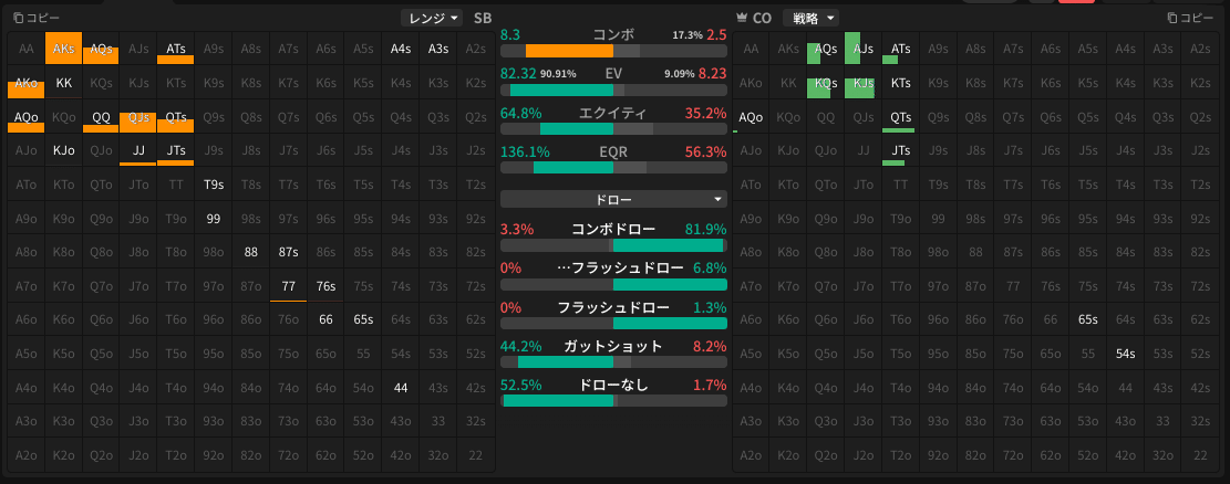
Consider the situation on a flop of KsTh5s (twotone board), where SB fires a 33% c-bet, CO calls, and the turn brings the Ah, creating a double flush-draw board [Figure 1].

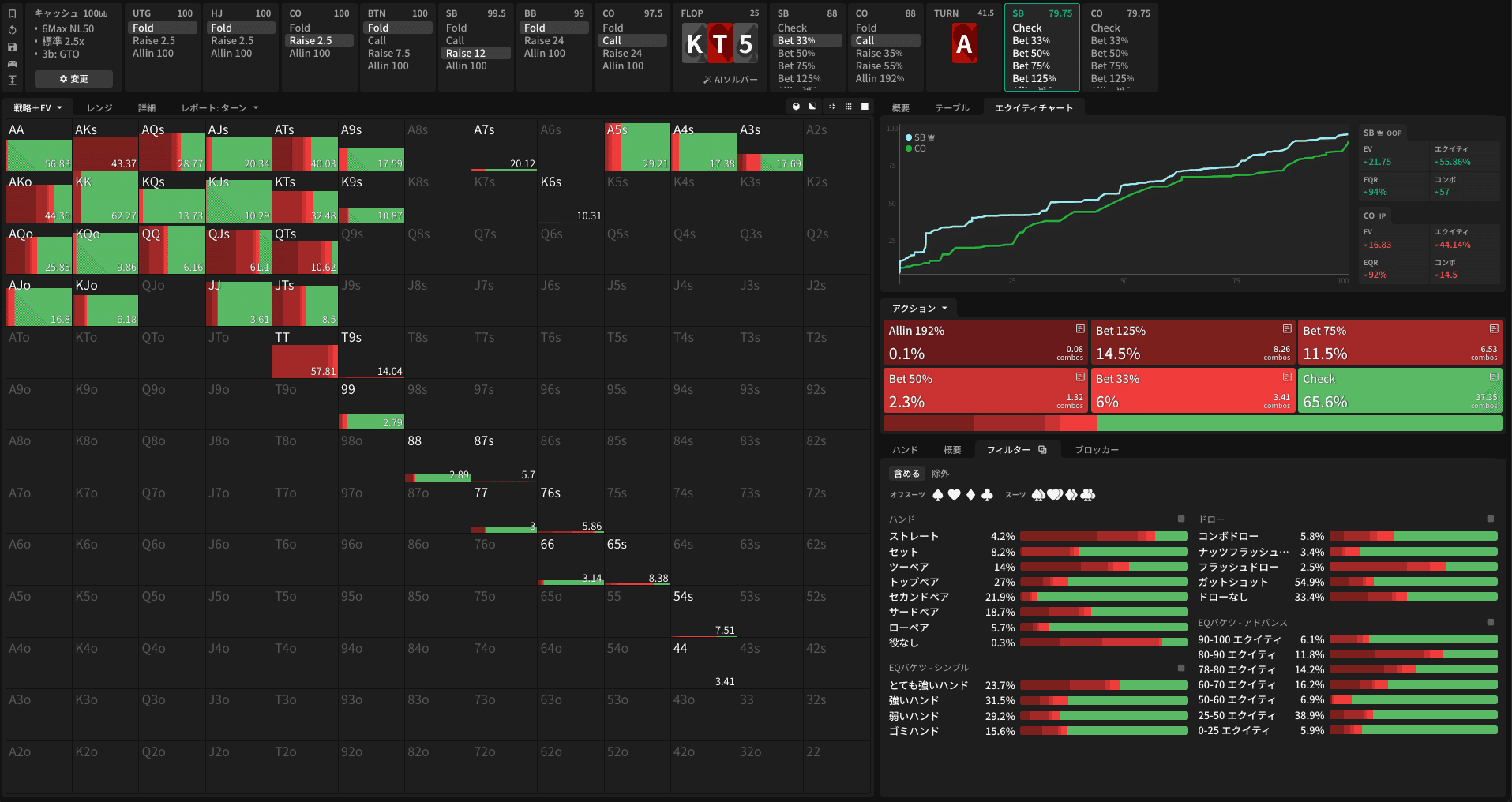
At this point on the turn, both players have an SPR of 1.92, and the 2-street geometric size (2e) for turn-river is 60.0%. In this spot, the b 75% and b 125% sizes are used at frequencies of 11.5% and 14.5% respectively as the primary sizes, making this a spot where hypergeometric sizing is employed.

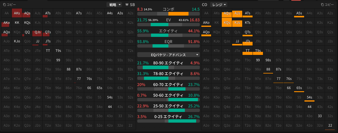
Looking at the EQ buckets at the start of the turn in Figure 2, hands with 70%+ equity (two pair, sets, straights) are held disproportionately by SB, while CO's range consists mostly of relatively marginal hands with lower equity (mostly hits or hit+draw combinations).

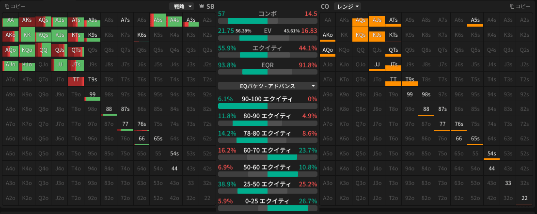
SB uses mainly two pair+ as value for b 125% (with certain considerations such as selecting only non-suited hands), and uses hands like TX with hit+GSSD as (semi-)bluffs. Against this b 125%, CO's hit+GSSD without a flush draw simply folds, and even hands like hit+FD+GSSD become indifferent between calling and folding (implied odds are extremely low against a large bet) [Figure 3].

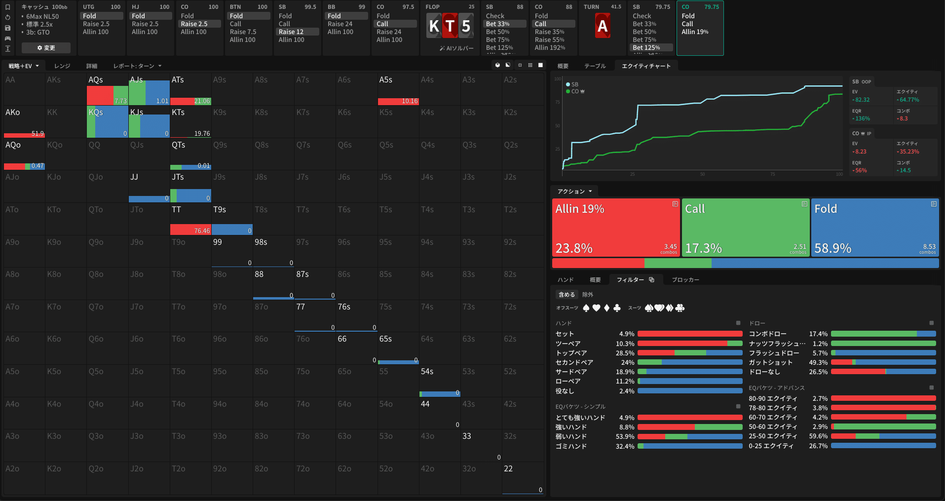
As can be seen from the EQ buckets in Figure 4, CO's calling range is composed almost entirely of combo draws. Focusing solely on flushes and roughly estimating the number of outs: half the range has a heart flush draw and the other half has a spade flush draw, each with 9 outs to complete the flush, giving $\frac{1}{2}\times18\,\%+\frac{1}{2}\times18\,\%=18\,\%$ probability that CO completes a draw on the river. When we also account for straight-completion outs, the probability of completing a draw is roughly 25% (a fairly rough estimate).

This spot is therefore analogous to the $S=2, p=1/4$ scenario we examined earlier. Restating the results:

$$ \begin{align*} r &= 1.422 \\ r' &= 0.1503 \end{align*} $$

and the corresponding bluff frequency $x$ is:

$$ \begin{align*} x=0.2784 \end{align*} $$

First, the appropriate bet sizes derived from the model are turn 142.2% – river 15.03%, which supports the GTO solution's main line of turn 125% – river 19%. Furthermore, the model's turn bluff frequency of 27.84% is very close to the GTO solution's turn bluff frequency ($\sim 26.4\,\%$) (counting hands below 50% equity as bluffs). In general, the larger the bet size, the more bluffs need to be included, but in draw-heavy situations like this, the bluff frequency can actually be lower than usual (the alpha, i.e., bluff frequency, for b 125% is 55.5%).

Summarizing the above observations: when IP has draws, it can be beneficial for OOP to use hypergeometric sizing to deny equity from IP's draw hands, thereby mitigating the disadvantage of being out of position.

Of course, there are many differences between the model and the actual GTO solution for this spot (for example, CO's raise all in on the turn), and a more refined model would need to account for OOP (SB)'s marginal hands and IP's high-equity hands, among other factors. However, despite being a simple model solvable by hand (with some assistance from numerical computation), it successfully reproduces the situations where hypergeometric sizing is used and proves to be highly informative.